Tutorial
1. Introduction
A time series is a sequence of observations, or data points, that is arranged based on the times of their occurrence. The hourly measurement of wind speeds in meteorology, the minute by minute recording of electrical activity along the scalp in electroencephalography, and the weekly changes of stock prices in finances are just some examples of time series, among many others.
Some of the following properties may be observed in time series data [gutsequential]:
the data is not generated independently
their dispersion varies in time
they are often governed by a trend and/or have cyclic components
The study and analysis of time series can have multiple ends: to gain a better understanding of the mechanism generating the data, to predict future outcomes and behaviors, to classify and characterize events, or more.
[2]:
ts_anim()
[2]:
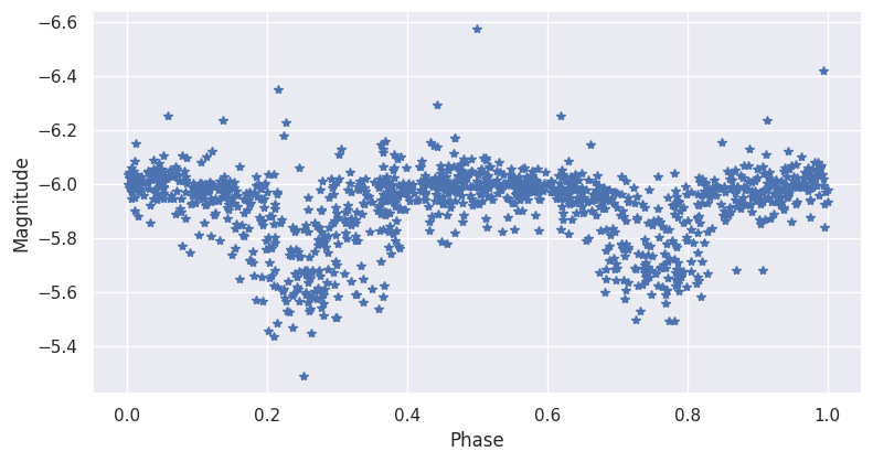
In time-domain astronomy, data gathered from telescopes is usually represented in the form of light curves, which are time series that show the brightness variation of an object over a period of time (for a visual representation, see the video below). Based on the variability characteristics of the light curves, celestial objects can be classified into different groups (quasars, long-period variables, eclipsing binaries, etc.) and consequently studied in depth independently.
Classification of data into groups can be performed in several ways given light curve data. Primarily, existing methods found in the literature use machine learning algorithms that group light curves into categories through feature extraction from the light curve data. These light curve features—the topic of this work—are numerical or categorical properties of the light curves that can be used to characterize and distinguish the different variability classes. Features can range from basic statistical properties such as the mean or standard deviation to more complex time series characteristics such as the autocorrelation function. Ideally, these features should be informative and discriminative, allowing machine learning or other algorithms to use them to distinguish between classes of light curves.
This document describes a tool that allows for the fast and efficient calculation of a compilation of many existing light curve features. The main goal is to create a collaborative and open tool where users can characterize or analyze an astronomical photometric database while also contributing to the library by adding new features. However, it is important to highlight that this library is not necessarily restricted to the astronomical domain and can also be applied to any kind of time series data.
Our vision is to be able to analyze and compare light curves from any available astronomical catalog in a standard and universal way. This would facilitate and make more efficient tasks such as modeling, classification, data cleaning, outlier detection, and data analysis in general. Consequently, when studying light curves, astronomers and data analysts using our library would be able to compare and match different features in a standardized way. To achieve this goal, the library should be run and features generated for every existing survey (MACHO, EROS, OGLE, Catalina, Pan-STARRS, VVV, etc.), as well as for future surveys (LSST), and the results shared openly, as is this library.
In the remainder of this document, we provide an overview of the features developed so far and explain how users can contribute to the library. A README file is also available for extra information.
Video 1: Light-curve of triple star
The video below shows how data from the brightness intensity of a star through time results on a light-curve. In this particular case we are observing a complex triple system in which three stars have mutual eclipses as each of the stars gets behind or in front of the others.
[3]:
macho_video()
[3]:
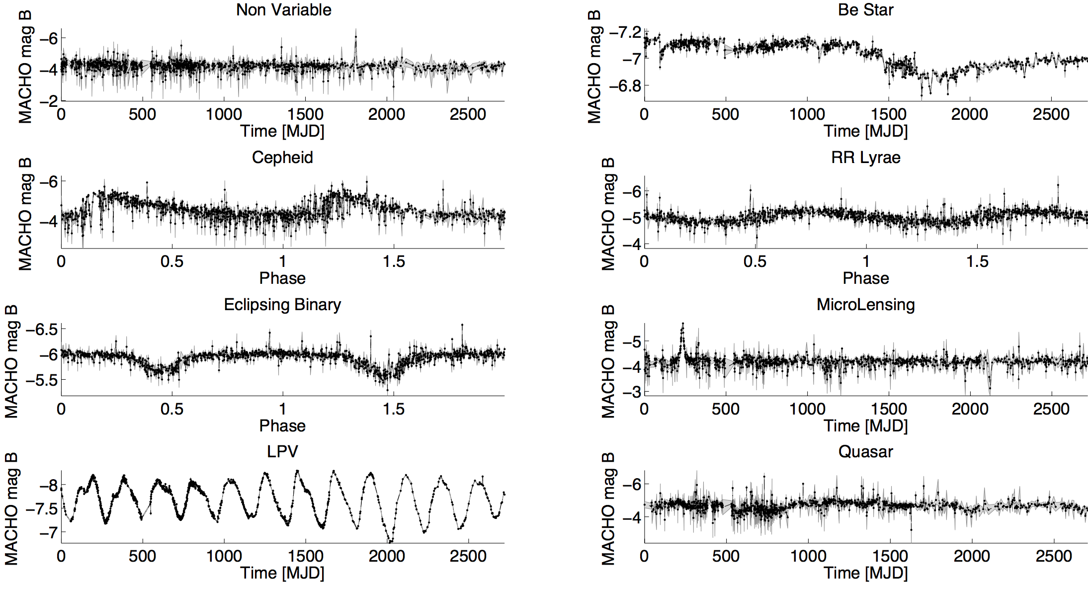
The following figure presents example light-curves of each class in the MACHO survey. The x-axis is the modified Julian Date (MJD), and the y-axis is the MACHO B-magnitude.
[4]:
macho_example11()
[4]:
2. The library
feets (feATURE eXTRACTOR FOR tIME sERIES) is a Python library designed for fast and efficient calculation of a wide range of light-curve features.
You can install the library directly from PyPI using pip:
pip install feets
Alternatively, you can download the source code or contribute new features via pull requests on GitHub: https://github.com/quatrope/feets. For a quick guide to using GitHub, visit https://guides.github.com/activities/hello-world/.
Input data vectors
The library accepts time series data vectors as input, and returns the calculated features as output. The set of features that can be computed depends on the available input vectors. For example, if only magnitude and time are provided, only features requiring those vectors will be calculated.
To compute all possible features, the following vectors (also referred to as raw data) are needed for each light curve:
timemagnitudeerrortime2magnitude2error2fluxflux_error
Here, the suffix 2 indicates a different observation band.
Below is an example of how the input might look if you have only magnitude and time vectors available:
[5]:
lc_example = np.array([time_ex, magnitude_ex])
lc_example
[5]:
array([[0.00000000e+00, 1.00000000e+00, 2.00000000e+00, 3.00000000e+00,
        4.00000000e+00, 5.00000000e+00, 6.00000000e+00, 7.00000000e+00,
        8.00000000e+00, 9.00000000e+00, 1.00000000e+01, 1.10000000e+01,
        1.20000000e+01, 1.30000000e+01, 1.40000000e+01, 1.50000000e+01,
        1.60000000e+01, 1.70000000e+01, 1.80000000e+01, 1.90000000e+01,
        2.00000000e+01, 2.10000000e+01, 2.20000000e+01, 2.30000000e+01,
        2.40000000e+01, 2.50000000e+01, 2.60000000e+01, 2.70000000e+01,
        2.80000000e+01, 2.90000000e+01],
       [1.52512421e-01, 6.91870898e-01, 3.51065233e-01, 1.70651992e-03,
        7.40076851e-01, 3.09347390e-01, 8.58862629e-02, 4.55181604e-02,
        3.21153924e-02, 5.18202896e-01, 9.70619463e-01, 9.53391511e-01,
        6.90576675e-01, 7.59149975e-01, 7.70791375e-01, 6.33311579e-02,
        8.09513022e-01, 7.45320879e-01, 8.33692892e-01, 6.08258035e-01,
        6.82890305e-01, 6.29338787e-01, 9.73110118e-02, 5.99520419e-01,
        2.66047089e-01, 2.76743822e-01, 9.62053925e-01, 5.10085356e-01,
        9.39188979e-01, 8.85351149e-01]])
When observed in different bands, light curves of a same object are not always monitored for the same time length and at the same precise times. For some features, it is important to align the light curves and to only consider the simultaneous measurements from both bands. The aligned vectors refer to the arrays obtained by synchronizing the raw data.
Thus, the actual input needed by the library is a dictionary containing the following vectors:
timemagnitudeerrorfluxflux_errormagnitude2aligned_timealigned_magnitudealigned_magnitude2aligned_erroraligned_error2
Not every data vector is required for every feature: the specific requirements depend on the features you choose to calculate. The more data vectors you provide, the more features that can be extracted. While the magnitude is the most commonly used input, some features require flux or other vectors. At least one data vector must be supplied to compute any feature.
Library structure
The library is divided into two main parts:
feets.FeatureSpace: A wrapper class that allows you to select the features to be calculated based on the available time series vectors or by specifying a list of features. This is the main entry point for usingfeets.feets.extractors: A package containing the actual code for calculating the features, and multiple tools to create your own extractor. Each feature has its own extractor class, and every extractor can compute at least one feature.
3. Reading an example light-curve
feets includes functionalities to download and read light curves from the existing catalogs of MACHO and OGLE-III.
MACHO
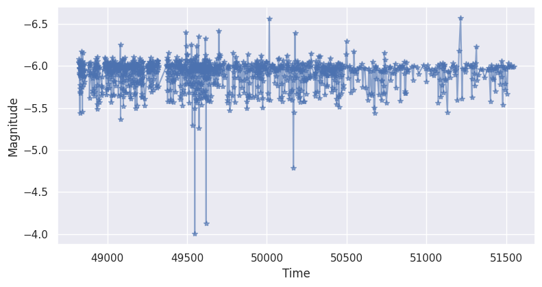
You can load an example light curve from the MACHO survey.
[6]:
from feets.datasets import macho

macho_dataset = macho.load_MACHO_example()
print("ID:", macho_dataset._id)
print("Bands:", macho_dataset.bands)

# Visualize the light curve for the B band
import matplotlib.pyplot as plt
plt.plot(macho_dataset.data.B.time, macho_dataset.data.B.magnitude, "*-", alpha=0.6)
plt.xlabel("Time")
plt.ylabel("Magnitude")
plt.gca().invert_yaxis()
plt.show()
ID: lc_1.3444.614
Bands: ('R', 'B')
OGLE-III
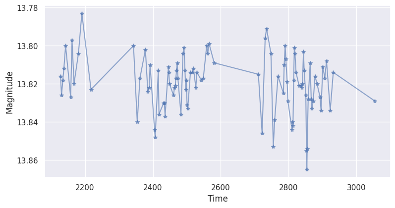
You can also fetch light curves from the OGLE-III catalog by providing a valid ID.
[7]:
from feets.datasets import ogle3

# This will download the data if not found locally
ogle3_dataset = ogle3.fetch_OGLE3("OGLE-BLG-LPV-232377")
print("ID:", ogle3_dataset._id)
print("Bands:", ogle3_dataset.bands)


# Visualize the light curve for the I band
import matplotlib.pyplot as plt
plt.plot(ogle3_dataset.data.I.time, ogle3_dataset.data.I.magnitude, "*-", alpha=0.6)
plt.xlabel("Time")
plt.ylabel("Magnitude")
plt.gca().invert_yaxis()
plt.show()
ID: OGLE-BLG-LPV-232377
Bands: ('V', 'I')
4. Preprocessing
Before feature extraction, it’s common to preprocess the data. feets provides tools for:
Removing noise: Points beyond a certain standard deviation from the mean are eliminated.
Aligning: Synchronizes light curves from two different bands for simultaneous measurements.
[8]:
import feets.preprocess

# Use the raw MACHO light curve from the previous step
b_band = macho_dataset.data.B
r_band = macho_dataset.data.R

# Remove noise from the data
time, mag, error = feets.preprocess.remove_noise(
    time=b_band.time,
    magnitude=b_band.magnitude,
    error=b_band.error,
)
time2, mag2, error2 = feets.preprocess.remove_noise(
    time=r_band.time,
    magnitude=r_band.magnitude,
    error=r_band.error,
)

# Synchronize the data from the two bands
atime, amag, amag2, aerror, aerror2 = feets.preprocess.align(
    time, time2, mag, mag2, error, error2
)

# For convenience, we store the preprocessed data in a dictionary.
lc = {
    "time": time,
    "magnitude": mag,
    "error": error,
    "magnitude2": mag2,
    "time2": time2,
    "error2": error2,
    "aligned_time": atime,
    "aligned_magnitude": amag,
    "aligned_magnitude2": amag2,
    "aligned_error": aerror,
    "aligned_error2": aerror2,
}

print(lc)
{'time': array([48823.477419, 48823.487014, 48823.496759, ..., 51531.401331,
51541.344537, 51546.325197], shape=(1194,)), 'magnitude': array([-6.081, -6.041, -6.046, ..., -6.009, -5.985, -5.997], shape=(1194,)), 'error': array([0.156, 0.141, 0.167, ..., 0.043, 0.024, 0.027], shape=(1194,)), 'magnitude2': array([-5.726, -6.09 , -5.751, -5.455, -5.561, -5.593, -5.732, -5.584,
-5.66 , -5.667, -5.037, -5.423, -5.431, -5.56 , -5.73 , -6.409,
-5.755, -5.584, -5.786, -5.591, -5.648, -5.849, -5.638, -5.636,
-5.642, -5.649, -5.748, -5.733, -5.849, -5.719, -5.477, -5.385,
-5.446, -5.253, -5.552, -5.117, -5.283, -5.759, -5.544, -5.722,
-5.717, -5.643, -5.622, -5.686, -5.709, -5.477, -5.562, -5.614,
-5.606, -5.689, -5.213, -5.58 , -5.736, -5.698, -5.759, -5.281,
-5.271, -5.432, -5.854, -5.682, -5.786, -5.659, -5.698, -5.529,
-5.393, -5.248, -5.693, -5.521, -5.649, -5.621, -5.629, -5.637,
-5.64 , -5.849, -5.558, -5.719, -5.543, -5.574, -6.139, -5.597,
-5.526, -5.726, -5.665, -5.717, -5.695, -5.8 , -5.58 , -5.248,
-5.549, -5.372, -5.524, -5.541, -5.333, -5.586, -5.464, -5.639,
-5.678, -5.692, -5.628, -5.678, -5.606, -5.651, -5.676, -5.639,
-5.378, -5.265, -5.498, -5.594, -5.62 , -5.715, -5.602, -5.677,
-5.688, -5.565, -5.647, -5.6 , -5.286, -5.532, -5.651, -5.583,
-5.638, -5.69 , -5.59 , -5.686, -5.164, -5.735, -5.68 , -5.648,
-5.641, -5.272, -5.56 , -5.649, -5.611, -5.76 , -5.718, -5.6 ,
-5.604, -5.627, -5.623, -5.656, -5.65 , -5.592, -5.671, -5.595,
-5.688, -5.731, -5.698, -5.18 , -5.391, -5.847, -5.604, -5.665,
-5.862, -5.566, -5.624, -5.649, -5.68 , -5.64 , -5.722, -5.701,
-5.457, -5.269, -5.648, -5.665, -5.544, -5.561, -5.581, -5.685,
-5.605, -5.389, -5.558, -5.484, -5.371, -5.438, -5.5 , -5.483,
-5.698, -5.694, -5.687, -5.819, -5.54 , -5.515, -5.657, -5.638,
-5.701, -5.645, -5.653, -6.029, -5.661, -6.064, -5.207, -5.267,
-5.605, -5.63 , -5.552, -5.589, -5.548, -5.614, -5.679, -5.12 ,
-5.169, -5.606, -5.633, -5.594, -5.645, -5.584, -5.618, -5.577,
-5.516, -5.278, -5.637, -5.68 , -5.43 , -5.591, -5.723, -5.591,
-5.811, -5.855, -5.626, -5.681, -5.534, -5.377, -5.635, -5.711,
-5.589, -5.559, -5.691, -5.476, -5.581, -5.512, -5.388, -5.692,
-5.633, -5.654, -5.373, -5.338, -5.535, -5.65 , -5.662, -5.559,
-5.583, -5.666, -5.634, -5.637, -5.654, -5.634, -5.556, -5.621,
-5.635, -5.621, -5.151, -5.465, -5.642, -5.141, -5.47 , -5.596,
-5.616, -5.638, -5.67 , -5.53 , -5.65 , -5.662, -5.69 , -5.673,
-5.529, -5.631, -5.616, -5.999, -5.552, -5.248, -5.494, -5.75 ,
-5.745, -5.85 , -5.646, -5.655, -5.68 , -5.553, -5.555, -5.626,
-5.591, -5.7 , -5.631, -5.956, -5.777, -5.585, -5.575, -5.203,
-5.549, -5.681, -5.683, -5.67 , -5.621, -5.667, -5.788, -5.428,
-5.487, -5.426, -5.167, -5.562, -5.34 , -5.375, -5.337, -5.244,
-5.598, -6.012, -5.994, -5.629, -5.58 , -5.6 , -5.623, -5.652,
-5.659, -5.548, -5.738, -5.577, -5.481, -5.609, -5.418, -5.629,
-5.401, -5.522, -5.398, -5.809, -5.332, -5.646, -5.636, -5.61 ,
-5.651, -5.604, -5.618, -5.612, -5.639, -5.631, -5.723, -5.706,
-5.465, -5.291, -5.133, -5.496, -5.469, -5.548, -5.556, -5.693,
-5.622, -5.653, -5.736, -5.667, -5.351, -5.463, -5.328, -5.537,
-5.637, -5.507, -5.679, -5.724, -5.758, -5.764, -5.477, -5.565,
-6.001, -5.578, -5.649, -5.427, -5.58 , -5.713, -5.802, -5.626,
-5.651, -5.632, -5.618, -5.707, -5.696, -5.593, -5.413, -5.208,
-5.552, -5.62 , -5.592, -5.647, -5.616, -5.592, -5.645, -5.651,
-5.57 , -5.222, -5.485, -5.344, -5.638, -5.634, -5.682, -5.609,
-5.354, -5.388, -5.417, -5.647, -5.727, -5.621, -5.572, -5.671,
-5.656, -5.68 , -5.471, -5.609, -5.616, -5.668, -5.664, -5.584,
-5.61 , -5.386, -5.435, -5.531, -5.611, -5.6 , -5.603, -5.831,
-5.71 , -5.641, -5.689, -5.696, -5.74 , -5.659, -5.386, -5.584,
-5.212, -5.627, -5.596, -5.671, -5.149, -5.798, -5.649, -5.616,
-5.779, -5.221, -5.645, -5.608, -5.689, -5.675, -5.592, -5.811,
-5.601, -5.575, -5.53 , -5.516, -5.32 , -5.346, -5.461, -5.67 ,
-5.633, -5.667, -5.599, -5.853, -5.615, -5.597, -5.701, -5.66 ,
-5.629, -5.521, -5.363, -5.534, -5.784, -5.561, -5.629, -5.584,
-5.583, -5.425, -5.616, -5.435, -5.37 , -5.658, -5.612, -5.585,
-5.557, -5.544, -5.621, -5.708, -5.616, -5.819, -5.605, -5.601,
-5.244, -5.307, -5.625, -5.647, -5.196, -5.543, -5.632, -5.83 ,
-5.623, -5.66 , -5.632, -5.629, -5.788, -5.62 , -5.683, -5.625,
-5.348, -5.689, -5.615, -5.693, -5.76 , -5.667, -5.415, -5.609,
-5.7 , -5.642, -5.562, -5.634, -5.652, -5.289, -5.609, -5.21 ,
-5.636, -5.401, -5.731, -5.663, -5.747, -5.725, -5.601, -5.574,
-5.69 , -5.721, -5.778, -5.61 , -5.305, -5.692, -5.637, -5.583,
-5.632, -5.775, -5.634, -5.718, -5.352, -5.664, -5.62 , -5.502,
-5.813, -5.249, -5.498, -5.55 , -5.621, -5.645, -5.635, -5.582,
-5.51 , -5.436, -5.535, -5.638, -5.658, -5.586, -5.599, -5.512,
-5.516, -5.662, -5.628, -5.783, -5.599, -5.651, -5.603, -5.552,
-5.482, -5.588, -5.223, -5.519, -5.405, -5.602, -5.634, -5.695,
-5.595, -5.653, -5.586, -5.621, -5.713, -5.711, -5.622, -5.611,
-5.513, -5.537, -5.338, -5.426, -5.668, -5.613, -5.649, -5.622,
-5.634, -5.616, -5.573, -5.535, -5.514, -5.611, -5.611, -5.649,
-5.633, -5.3 , -5.278, -5.528, -5.19 , -5.56 , -5.612, -5.633,
-5.37 , -5.642, -5.367, -5.38 , -5.705, -5.62 , -5.291, -5.763,
-5.553, -5.591, -5.589, -5.548, -5.561, -5.361, -5.533, -5.637,
-5.22 , -5.384, -5.489, -5.595, -5.581, -5.63 , -5.547, -5.31 ,
-5.617, -5.516, -5.642, -5.655, -5.627, -5.66 , -5.579, -5.391,
-5.596, -5.666, -5.652, -5.52 , -5.659, -5.382, -5.459, -5.646,
-5.741, -5.529, -5.475, -5.595, -5.674, -5.532, -5.627, -5.677,
-5.652, -5.619, -5.549, -5.699, -5.162, -5.588, -5.719, -5.59 ,
-5.338, -5.675, -5.588, -5.512, -5.416, -5.605, -5.622, -5.659,
-5.381, -5.482, -5.572, -5.644, -5.561, -5.636, -5.595, -5.725,
-5.638, -5.642, -5.634, -5.605, -5.225, -5.538, -5.646, -5.622,
-5.537, -5.624, -5.661, -5.333, -5.652, -5.586, -5.635, -5.579,
-5.534, -5.509, -5.597, -5.638, -5.608, -5.614, -5.217, -5.557,
-5.64 , -5.608, -5.418, -5.594, -5.737, -5.24 , -5.652, -5.593,
-5.708, -5.598, -5.626]), 'time2': array([48823.487014, 48823.496759, 48824.458206, 48824.467697,
48824.477639, 48825.483183, 48825.492847, 48825.502824,
48826.46463 , 48826.491319, 48828.585961, 48828.656701,
48829.456285, 48829.584769, 48829.659965, 48831.461817,
48831.564722, 48831.63897 , 48831.661551, 48832.459769,
48832.65125 , 48833.569375, 48834.430926, 48834.515544,
48834.639225, 48835.571053, 48835.606296, 48836.564236,
48841.441516, 48841.541134, 48841.633623, 48842.458345,
48842.565046, 48842.632581, 48843.416875, 48843.562419,
48843.64015 , 48849.5836 , 48850.497442, 48851.481181,
48851.59765 , 48853.645799, 48854.557338, 48855.527002,
48855.579722, 48856.609769, 48882.423356, 48884.469873,
48885.43728 , 48887.500475, 48888.555648, 48892.592604,
48894.561655, 48895.587106, 48896.589398, 48906.407998,
48907.393912, 48908.278576, 48909.39735 , 48914.57809 ,
48915.430718, 48916.516921, 48917.352616, 48919.355104,
48919.441273, 48919.516227, 48919.599155, 48920.286863,
48923.513403, 48927.261887, 48928.290602, 48929.238299,
48929.449583, 48930.241771, 48931.239676, 48931.425579,
48933.393738, 48935.39787 , 48937.415289, 48937.43831 ,
48938.280475, 48939.296157, 48939.460255, 48941.356863,
48941.48287 , 48947.395671, 48947.518785, 48948.477627,
48949.293924, 48964.443623, 48965.279294, 48965.417766,
48966.282199, 48966.397812, 48974.325278, 48984.27625 ,
48985.303611, 48985.432188, 48987.291701, 48987.420023,
48988.279826, 48988.402917, 48988.421447, 48989.301412,
48989.40787 , 48996.248657, 48996.36287 , 48998.250903,
48998.360602, 49000.265278, 49001.253808, 49002.251262,
49003.34735 , 49004.244248, 49006.260463, 49007.268877,
49010.352685, 49011.340336, 49015.25419 , 49016.253032,
49018.277998, 49020.335648, 49021.28294 , 49024.250046,
49025.28228 , 49029.25066 , 49031.271181, 49032.246528,
49037.232407, 49040.268785, 49043.24875 , 49044.258819,
49045.232731, 49048.229363, 49049.245069, 49051.225023,
49059.226759, 49060.209271, 49061.212512, 49062.21044 ,
49067.204433, 49069.206516, 49073.203194, 49074.196262,
49075.18831 , 49083.215868, 49134.663275, 49140.62162 ,
49141.622037, 49142.605845, 49143.606806, 49144.624734,
49151.608009, 49152.604005, 49161.607766, 49162.580833,
49163.60213 , 49163.615428, 49164.58853 , 49165.565984,
49167.678912, 49169.604664, 49178.587569, 49179.548056,
49180.515961, 49181.506146, 49181.661898, 49182.601771,
49183.495266, 49183.656319, 49184.488773, 49185.500185,
49186.510347, 49186.600104, 49188.483866, 49189.492315,
49194.506377, 49194.670336, 49195.455972, 49196.490359,
49199.517847, 49203.474479, 49204.47309 , 49208.461794,
49209.440972, 49210.459005, 49211.490463, 49212.603762,
49215.431887, 49216.418785, 49217.427801, 49218.417963,
49219.434456, 49220.525185, 49221.414838, 49222.399861,
49223.401736, 49224.387338, 49225.607593, 49233.381319,
49233.412257, 49252.368484, 49253.374977, 49254.430914,
49255.348565, 49256.361285, 49257.35706 , 49258.316123,
49258.53647 , 49259.520359, 49260.341319, 49264.530856,
49265.316053, 49266.396713, 49267.412257, 49268.371898,
49269.411806, 49270.374954, 49272.406273, 49273.289282,
49276.55794 , 49277.446852, 49279.537894, 49280.495324,
49282.344294, 49283.271343, 49285.468495, 49286.282083,
49287.361389, 49289.366065, 49290.569097, 49291.256968,
49302.360058, 49303.214641, 49307.291134, 49309.253981,
49311.303021, 49312.315012, 49313.270556, 49314.242569,
49315.268507, 49317.270243, 49318.402569, 49372.256748,
49375.265961, 49376.287199, 49378.241701, 49380.243715,
49386.266238, 49390.256655, 49398.232836, 49399.237361,
49400.256956, 49413.230787, 49414.246736, 49415.230278,
49416.222951, 49417.228715, 49423.211713, 49426.216516,
49432.217963, 49487.657442, 49488.648333, 49491.638252,
49493.632824, 49494.640451, 49496.634977, 49500.662118,
49511.603032, 49512.597743, 49513.642245, 49517.563102,
49518.574329, 49518.584155, 49520.580926, 49521.659954,
49522.590336, 49525.618044, 49530.650521, 49531.571065,
49532.643148, 49534.609757, 49535.666181, 49537.653044,
49538.613183, 49539.619271, 49540.600035, 49541.607407,
49545.505961, 49546.50434 , 49546.66478 , 49550.642002,
49551.620637, 49552.672813, 49553.463125, 49554.474803,
49554.670185, 49555.5114 , 49555.650775, 49556.515694,
49556.652164, 49557.598368, 49558.548252, 49559.483356,
49559.660023, 49560.529965, 49560.669664, 49561.540579,
49562.571782, 49566.465613, 49566.651667, 49567.502662,
49567.65875 , 49568.540208, 49568.655775, 49569.508345,
49569.658021, 49571.472593, 49571.65985 , 49572.479294,
49572.492743, 49572.655312, 49573.470069, 49574.47088 ,
49574.506725, 49577.450046, 49577.64081 , 49578.462928,
49578.640104, 49579.47162 , 49579.635313, 49580.42772 ,
49580.644201, 49581.477373, 49585.457824, 49586.463229,
49587.461227, 49588.497789, 49589.427639, 49589.501157,
49590.43566 , 49591.458102, 49592.427187, 49595.463808,
49596.456875, 49597.525046, 49598.488704, 49599.492442,
49601.566019, 49602.448519, 49604.465787, 49605.454722,
49606.458333, 49607.334745, 49608.459375, 49609.485799,
49610.43956 , 49611.44544 , 49612.442604, 49613.617975,
49614.445602, 49616.469907, 49617.424745, 49618.422975,
49620.455741, 49621.566123, 49622.454387, 49623.453935,
49624.619896, 49625.435903, 49627.442859, 49628.49478 ,
49629.496192, 49630.418403, 49633.364213, 49634.353623,
49635.423981, 49636.394769, 49637.476331, 49638.451065,
49639.399329, 49640.433588, 49641.543287, 49642.343148,
49645.324005, 49647.533079, 49648.334387, 49649.330694,
49651.453623, 49653.393981, 49654.359919, 49660.436725,
49664.478218, 49665.333646, 49666.287361, 49667.415822,
49670.306794, 49671.266678, 49672.243854, 49673.356007,
49674.490833, 49676.306979, 49681.29191 , 49682.310359,
49687.295926, 49688.30809 , 49689.372025, 49690.299375,
49691.344016, 49692.365949, 49693.317627, 49695.347037,
49696.342384, 49697.362593, 49698.467141, 49699.47853 ,
49700.309792, 49702.322581, 49703.392674, 49704.317535,
49705.381458, 49715.2764 , 49723.303125, 49727.280833,
49883.671562, 49901.667627, 49905.641829, 49907.633657,
49912.645428, 49916.661736, 49917.610382, 49921.552639,
49927.471157, 49929.56 , 49931.629039, 49933.468576,
49935.583218, 49936.571076, 49937.586053, 49938.456979,
49939.483796, 49940.621991, 49941.465301, 49942.537986,
49943.530891, 49944.553102, 49945.536076, 49946.6225 ,
49947.625185, 49948.572234, 49949.429433, 49951.449595,
49952.529676, 49953.4464 , 49954.534132, 49955.621678,
49957.399525, 49958.651366, 49961.412928, 49963.594375,
49965.458472, 49966.511157, 49967.406146, 49969.372153,
49970.369016, 49971.638762, 49972.382523, 49973.617662,
49974.58522 , 49980.410174, 49982.345081, 49986.396597,
49987.355741, 49994.384502, 49994.591169, 49995.560822,
49996.418924, 49997.475694, 49998.499271, 50003.433958,
50005.414317, 50006.400417, 50007.482419, 50013.367569,
50019.431563, 50021.427106, 50022.459444, 50029.303681,
50031.341771, 50033.305185, 50038.379792, 50038.497442,
50044.288241, 50045.364687, 50046.350023, 50047.425162,
50048.404525, 50054.307326, 50057.329583, 50058.341435,
50061.340069, 50063.310532, 50066.343727, 50071.280058,
50072.342384, 50074.310822, 50077.3814 , 50088.32625 ,
50089.320174, 50091.352442, 50091.397766, 50095.346123,
50105.323831, 50239.614225, 50263.606863, 50271.673738,
50276.58662 , 50276.630868, 50278.531366, 50293.575972,
50296.587257, 50297.571493, 50300.48588 , 50301.640856,
50302.494236, 50303.644375, 50304.540035, 50305.650058,
50307.474398, 50308.553322, 50310.596296, 50311.551829,
50315.522326, 50319.613287, 50320.65066 , 50322.451262,
50327.576736, 50329.582963, 50333.468056, 50333.502755,
50335.508542, 50340.602083, 50341.470532, 50341.510822,
50346.553021, 50348.359016, 50349.473646, 50350.439861,
50352.399074, 50353.335069, 50359.408993, 50360.43603 ,
50364.327083, 50364.587326, 50366.428958, 50368.368183,
50369.38897 , 50370.372407, 50371.355532, 50374.373229,
50376.353032, 50376.594803, 50377.381829, 50379.399294,
50380.354086, 50384.385729, 50385.436146, 50385.440567,
50389.284641, 50394.528287, 50395.369919, 50396.480567,
50397.426898, 50399.43816 , 50401.424722, 50405.291933,
50406.291273, 50406.524664, 50407.324433, 50409.296065,
50410.372743, 50411.374387, 50416.480475, 50417.50015 ,
50419.286921, 50419.342755, 50420.339109, 50422.45103 ,
50424.297419, 50425.49044 , 50426.336042, 50428.412616,
50429.480602, 50436.396134, 50437.320799, 50438.360868,
50451.391343, 50607.641435, 50614.629676, 50639.547373,
50642.505359, 50647.56537 , 50656.612465, 50659.485463,
50661.623356, 50669.50375 , 50670.656597, 50675.471111,
50679.422627, 50680.600741, 50682.453773, 50684.616181,
50689.564086, 50701.557454, 50704.54147 , 50714.465521,
50717.550937, 50719.490475, 50721.385764, 50722.513032,
50725.33294 , 50730.411238, 50731.536539, 50733.405359,
50734.501377, 50736.366435, 50737.431053, 50739.340683,
50742.305613, 50744.511667, 50746.385914, 50748.359039,
50767.318912, 50769.392164, 50771.453843, 50775.478056,
50785.319896, 50796.309884, 50808.316435, 50812.365208,
50973.558808, 50994.63103 , 51000.587037, 51005.552847,
51017.536748, 51028.466447, 51033.648148, 51047.619815,
51051.538252, 51056.406933, 51061.467326, 51072.414873,
51073.585567, 51082.594711, 51085.362014, 51086.581412,
51089.466771, 51097.459722, 51099.576968, 51102.371123,
51106.435984, 51109.472373, 51111.477662, 51113.547731,
51118.432083, 51120.48103 , 51136.526806, 51141.342674,
51147.454086, 51156.269641, 51183.344514, 51188.24287 ,
51350.66985 , 51382.605521, 51389.617257, 51393.557442,
51401.545359, 51405.657141, 51408.601852, 51411.592847,
51414.526968, 51421.462396, 51424.478356, 51431.46713 ,
51433.593194, 51435.568542, 51440.429317, 51443.546042,
51450.408218, 51462.365278, 51463.537118, 51468.473854,
51471.379803, 51472.524039, 51478.35787 , 51479.490509,
51484.263657, 51488.448588, 51491.480567, 51493.515324,
51495.492697, 51505.470833, 51510.444271, 51513.293056,
51514.451319, 51526.316157, 51541.344537]), 'error2': array([0.181, 0.143, 0.073, 0.084, 0.076, 0.065, 0.061, 0.068, 0.106,
0.094, 0.132, 0.099, 0.06 , 0.166, 0.084, 0.144, 0.088, 0.046,
0.076, 0.094, 0.079, 0.096, 0.064, 0.051, 0.041, 0.111, 0.085,
0.196, 0.1 , 0.044, 0.059, 0.195, 0.074, 0.078, 0.154, 0.129,
0.09 , 0.077, 0.104, 0.097, 0.091, 0.068, 0.047, 0.042, 0.041,
0.053, 0.06 , 0.054, 0.035, 0.087, 0.064, 0.056, 0.067, 0.04 ,
0.038, 0.082, 0.124, 0.033, 0.105, 0.076, 0.09 , 0.053, 0.033,
0.039, 0.078, 0.086, 0.075, 0.056, 0.033, 0.056, 0.038, 0.057,
0.03 , 0.084, 0.054, 0.032, 0.048, 0.129, 0.209, 0.088, 0.055,
0.045, 0.053, 0.047, 0.047, 0.085, 0.094, 0.048, 0.034, 0.106,
0.11 , 0.076, 0.084, 0.066, 0.139, 0.045, 0.033, 0.036, 0.026,
0.04 , 0.043, 0.051, 0.051, 0.046, 0.18 , 0.052, 0.053, 0.03 ,
0.035, 0.045, 0.036, 0.029, 0.045, 0.038, 0.026, 0.072, 0.028,
0.097, 0.043, 0.047, 0.035, 0.057, 0.045, 0.081, 0.082, 0.051,
0.076, 0.063, 0.023, 0.053, 0.032, 0.053, 0.031, 0.057, 0.071,
0.047, 0.027, 0.028, 0.031, 0.04 , 0.045, 0.046, 0.051, 0.056,
0.055, 0.11 , 0.065, 0.156, 0.141, 0.176, 0.139, 0.099, 0.203,
0.066, 0.096, 0.104, 0.061, 0.052, 0.074, 0.098, 0.253, 0.105,
0.055, 0.071, 0.065, 0.122, 0.034, 0.073, 0.19 , 0.107, 0.093,
0.063, 0.16 , 0.104, 0.093, 0.09 , 0.074, 0.057, 0.073, 0.081,
0.082, 0.093, 0.065, 0.104, 0.105, 0.072, 0.054, 0.143, 0.178,
0.226, 0.049, 0.063, 0.152, 0.176, 0.09 , 0.036, 0.06 , 0.085,
0.05 , 0.239, 0.197, 0.045, 0.061, 0.038, 0.065, 0.048, 0.031,
0.106, 0.038, 0.086, 0.061, 0.08 , 0.096, 0.054, 0.073, 0.057,
0.079, 0.074, 0.035, 0.051, 0.036, 0.041, 0.056, 0.067, 0.041,
0.049, 0.112, 0.068, 0.052, 0.07 , 0.118, 0.068, 0.033, 0.041,
0.037, 0.036, 0.064, 0.033, 0.058, 0.09 , 0.042, 0.025, 0.083,
0.031, 0.052, 0.041, 0.093, 0.049, 0.046, 0.042, 0.037, 0.052,
0.063, 0.044, 0.042, 0.027, 0.026, 0.039, 0.082, 0.034, 0.042,
0.049, 0.223, 0.095, 0.274, 0.058, 0.171, 0.07 , 0.144, 0.16 ,
0.053, 0.104, 0.117, 0.166, 0.159, 0.085, 0.059, 0.11 , 0.08 ,
0.047, 0.042, 0.094, 0.035, 0.132, 0.082, 0.096, 0.091, 0.057,
0.072, 0.086, 0.048, 0.066, 0.03 , 0.035, 0.117, 0.135, 0.077,
0.204, 0.178, 0.074, 0.075, 0.1 , 0.177, 0.182, 0.043, 0.239,
0.202, 0.072, 0.05 , 0.1 , 0.035, 0.037, 0.038, 0.068, 0.084,
0.035, 0.045, 0.077, 0.139, 0.159, 0.143, 0.063, 0.081, 0.034,
0.032, 0.072, 0.057, 0.048, 0.027, 0.035, 0.021, 0.043, 0.037,
0.084, 0.081, 0.128, 0.086, 0.069, 0.058, 0.036, 0.041, 0.05 ,
0.083, 0.052, 0.031, 0.029, 0.056, 0.068, 0.083, 0.051, 0.036,
0.033, 0.03 , 0.177, 0.091, 0.06 , 0.087, 0.159, 0.126, 0.06 ,
0.22 , 0.062, 0.106, 0.093, 0.032, 0.067, 0.11 , 0.065, 0.078,
0.038, 0.058, 0.037, 0.074, 0.029, 0.048, 0.057, 0.056, 0.079,
0.029, 0.048, 0.029, 0.033, 0.026, 0.052, 0.091, 0.063, 0.048,
0.143, 0.043, 0.056, 0.079, 0.041, 0.066, 0.043, 0.05 , 0.041,
0.052, 0.098, 0.062, 0.064, 0.094, 0.094, 0.033, 0.046, 0.155,
0.048, 0.037, 0.022, 0.019, 0.022, 0.025, 0.061, 0.031, 0.019,
0.038, 0.133, 0.112, 0.062, 0.059, 0.077, 0.062, 0.081, 0.04 ,
0.042, 0.098, 0.03 , 0.043, 0.062, 0.163, 0.065, 0.069, 0.146,
0.071, 0.112, 0.07 , 0.041, 0.067, 0.057, 0.113, 0.092, 0.054,
0.047, 0.058, 0.026, 0.047, 0.06 , 0.156, 0.076, 0.021, 0.08 ,
0.058, 0.085, 0.031, 0.05 , 0.082, 0.081, 0.033, 0.149, 0.069,
0.096, 0.147, 0.04 , 0.061, 0.064, 0.075, 0.044, 0.05 , 0.112,
0.043, 0.086, 0.065, 0.043, 0.03 , 0.046, 0.039, 0.049, 0.043,
0.144, 0.044, 0.098, 0.031, 0.044, 0.06 , 0.05 , 0.068, 0.061,
0.07 , 0.103, 0.151, 0.041, 0.021, 0.031, 0.092, 0.042, 0.063,
0.071, 0.054, 0.05 , 0.121, 0.051, 0.042, 0.046, 0.031, 0.023,
0.063, 0.046, 0.019, 0.026, 0.032, 0.277, 0.025, 0.052, 0.047,
0.146, 0.073, 0.047, 0.039, 0.151, 0.062, 0.273, 0.08 , 0.073,
0.125, 0.065, 0.109, 0.063, 0.062, 0.052, 0.067, 0.072, 0.043,
0.085, 0.04 , 0.032, 0.084, 0.14 , 0.096, 0.098, 0.074, 0.176,
0.039, 0.056, 0.058, 0.051, 0.094, 0.182, 0.04 , 0.053, 0.109,
0.052, 0.028, 0.028, 0.08 , 0.054, 0.031, 0.098, 0.021, 0.031,
0.026, 0.041, 0.09 , 0.048, 0.033, 0.035, 0.123, 0.087, 0.061,
0.055, 0.04 , 0.03 , 0.03 , 0.042, 0.063, 0.059, 0.054, 0.031,
0.029, 0.037, 0.061, 0.067, 0.051, 0.043, 0.064, 0.065, 0.071,
0.041, 0.031, 0.038, 0.049, 0.033, 0.025, 0.036, 0.077, 0.064,
0.066, 0.066, 0.033, 0.04 , 0.088, 0.066, 0.062, 0.058, 0.082,
0.035, 0.08 , 0.035, 0.127, 0.231, 0.061, 0.036, 0.079, 0.221,
0.028, 0.029, 0.035, 0.038, 0.038, 0.054, 0.03 , 0.048, 0.056,
0.021, 0.087, 0.088, 0.063, 0.199, 0.101, 0.109, 0.045, 0.042,
0.039, 0.073, 0.037, 0.04 , 0.032, 0.1 , 0.037, 0.057, 0.098,
0.029, 0.229, 0.076, 0.05 , 0.082, 0.053, 0.075, 0.049, 0.038,
0.046, 0.054, 0.073, 0.07 , 0.071, 0.029, 0.08 , 0.113, 0.11 ,
0.21 , 0.167, 0.076, 0.095, 0.027, 0.121, 0.08 , 0.074, 0.054,
0.049, 0.036, 0.027, 0.035, 0.032, 0.05 , 0.055, 0.035, 0.099,
0.063, 0.061, 0.052, 0.052, 0.083, 0.037, 0.04 , 0.044, 0.127,
0.04 , 0.034, 0.05 , 0.048, 0.099, 0.147, 0.049, 0.038, 0.033,
0.051, 0.075, 0.037, 0.052, 0.024, 0.065, 0.03 , 0.045, 0.063,
0.024, 0.027, 0.04 , 0.026, 0.03 ]), 'aligned_time': array([48823.487014, 48823.496759, 48824.458206, 48824.467697,
48824.477639, 48825.483183, 48825.492847, 48825.502824,
48826.46463 , 48826.491319, 48828.585961, 48828.656701,
48829.456285, 48829.584769, 48829.659965, 48831.564722,
48831.63897 , 48831.661551, 48832.459769, 48832.65125 ,
48833.569375, 48834.430926, 48834.515544, 48834.639225,
48835.571053, 48835.606296, 48836.564236, 48841.441516,
48841.541134, 48842.458345, 48843.416875, 48843.562419,
48843.64015 , 48849.5836 , 48850.497442, 48851.481181,
48851.59765 , 48853.645799, 48854.557338, 48855.527002,
48855.579722, 48856.609769, 48882.423356, 48884.469873,
48885.43728 , 48887.500475, 48888.555648, 48892.592604,
48894.561655, 48895.587106, 48896.589398, 48906.407998,
48907.393912, 48908.278576, 48909.39735 , 48914.57809 ,
48915.430718, 48916.516921, 48917.352616, 48919.355104,
48919.441273, 48919.516227, 48919.599155, 48920.286863,
48923.513403, 48927.261887, 48928.290602, 48929.238299,
48929.449583, 48930.241771, 48931.239676, 48931.425579,
48933.393738, 48935.39787 , 48937.43831 , 48938.280475,
48939.296157, 48939.460255, 48941.356863, 48941.48287 ,
48947.395671, 48947.518785, 48948.477627, 48949.293924,
48964.443623, 48965.279294, 48965.417766, 48966.282199,
48966.397812, 48974.325278, 48984.27625 , 48985.303611,
48985.432188, 48987.291701, 48987.420023, 48988.279826,
48988.402917, 48988.421447, 48989.301412, 48989.40787 ,
48996.248657, 48996.36287 , 48998.250903, 48998.360602,
49000.265278, 49001.253808, 49002.251262, 49003.34735 ,
49004.244248, 49006.260463, 49007.268877, 49011.340336,
49015.25419 , 49016.253032, 49018.277998, 49020.335648,
49021.28294 , 49024.250046, 49025.28228 , 49029.25066 ,
49031.271181, 49032.246528, 49037.232407, 49040.268785,
49043.24875 , 49044.258819, 49045.232731, 49048.229363,
49049.245069, 49051.225023, 49059.226759, 49060.209271,
49061.212512, 49062.21044 , 49067.204433, 49069.206516,
49073.203194, 49074.196262, 49075.18831 , 49083.215868,
49134.663275, 49140.62162 , 49141.622037, 49142.605845,
49143.606806, 49144.624734, 49152.604005, 49161.607766,
49162.580833, 49163.60213 , 49163.615428, 49164.58853 ,
49165.565984, 49167.678912, 49169.604664, 49178.587569,
49179.548056, 49181.506146, 49181.661898, 49182.601771,
49183.495266, 49183.656319, 49184.488773, 49185.500185,
49186.510347, 49186.600104, 49188.483866, 49189.492315,
49194.506377, 49194.670336, 49195.455972, 49196.490359,
49199.517847, 49203.474479, 49204.47309 , 49208.461794,
49209.440972, 49210.459005, 49211.490463, 49212.603762,
49215.431887, 49217.427801, 49218.417963, 49219.434456,
49220.525185, 49221.414838, 49222.399861, 49223.401736,
49224.387338, 49225.607593, 49233.381319, 49233.412257,
49252.368484, 49253.374977, 49254.430914, 49255.348565,
49256.361285, 49257.35706 , 49258.316123, 49258.53647 ,
49259.520359, 49260.341319, 49264.530856, 49265.316053,
49266.396713, 49267.412257, 49268.371898, 49269.411806,
49270.374954, 49272.406273, 49273.289282, 49276.55794 ,
49277.446852, 49279.537894, 49280.495324, 49282.344294,
49283.271343, 49285.468495, 49286.282083, 49287.361389,
49289.366065, 49290.569097, 49291.256968, 49302.360058,
49303.214641, 49307.291134, 49309.253981, 49311.303021,
49312.315012, 49313.270556, 49314.242569, 49315.268507,
49317.270243, 49318.402569, 49372.256748, 49375.265961,
49376.287199, 49378.241701, 49380.243715, 49386.266238,
49390.256655, 49398.232836, 49399.237361, 49400.256956,
49413.230787, 49414.246736, 49415.230278, 49416.222951,
49417.228715, 49423.211713, 49426.216516, 49432.217963,
49487.657442, 49488.648333, 49491.638252, 49493.632824,
49494.640451, 49496.634977, 49500.662118, 49511.603032,
49512.597743, 49513.642245, 49517.563102, 49518.574329,
49518.584155, 49520.580926, 49521.659954, 49522.590336,
49525.618044, 49530.650521, 49531.571065, 49532.643148,
49534.609757, 49535.666181, 49537.653044, 49538.613183,
49539.619271, 49540.600035, 49541.607407, 49545.505961,
49546.50434 , 49546.66478 , 49550.642002, 49551.620637,
49552.672813, 49553.463125, 49554.474803, 49554.670185,
49555.5114 , 49555.650775, 49556.515694, 49556.652164,
49557.598368, 49558.548252, 49559.483356, 49559.660023,
49560.669664, 49561.540579, 49562.571782, 49566.465613,
49566.651667, 49567.502662, 49567.65875 , 49568.540208,
49568.655775, 49569.508345, 49569.658021, 49571.472593,
49571.65985 , 49572.479294, 49572.492743, 49572.655312,
49573.470069, 49574.47088 , 49574.506725, 49577.450046,
49577.64081 , 49578.462928, 49578.640104, 49579.47162 ,
49579.635313, 49580.42772 , 49580.644201, 49585.457824,
49586.463229, 49587.461227, 49588.497789, 49589.427639,
49589.501157, 49590.43566 , 49591.458102, 49592.427187,
49595.463808, 49596.456875, 49597.525046, 49598.488704,
49599.492442, 49601.566019, 49602.448519, 49604.465787,
49605.454722, 49606.458333, 49607.334745, 49608.459375,
49609.485799, 49610.43956 , 49611.44544 , 49612.442604,
49613.617975, 49616.469907, 49617.424745, 49618.422975,
49620.455741, 49621.566123, 49622.454387, 49623.453935,
49624.619896, 49625.435903, 49627.442859, 49628.49478 ,
49629.496192, 49630.418403, 49633.364213, 49634.353623,
49635.423981, 49636.394769, 49637.476331, 49638.451065,
49639.399329, 49640.433588, 49641.543287, 49642.343148,
49645.324005, 49647.533079, 49648.334387, 49649.330694,
49653.393981, 49654.359919, 49660.436725, 49664.478218,
49665.333646, 49666.287361, 49667.415822, 49670.306794,
49671.266678, 49672.243854, 49673.356007, 49674.490833,
49676.306979, 49681.29191 , 49682.310359, 49687.295926,
49688.30809 , 49689.372025, 49690.299375, 49691.344016,
49692.365949, 49693.317627, 49695.347037, 49696.342384,
49697.362593, 49698.467141, 49699.47853 , 49700.309792,
49702.322581, 49703.392674, 49704.317535, 49705.381458,
49715.2764 , 49723.303125, 49727.280833, 49883.671562,
49901.667627, 49905.641829, 49907.633657, 49912.645428,
49916.661736, 49917.610382, 49921.552639, 49927.471157,
49929.56 , 49931.629039, 49933.468576, 49935.583218,
49936.571076, 49937.586053, 49938.456979, 49939.483796,
49940.621991, 49941.465301, 49942.537986, 49943.530891,
49944.553102, 49945.536076, 49946.6225 , 49948.572234,
49949.429433, 49951.449595, 49952.529676, 49953.4464 ,
49954.534132, 49955.621678, 49957.399525, 49958.651366,
49961.412928, 49963.594375, 49965.458472, 49966.511157,
49967.406146, 49969.372153, 49970.369016, 49971.638762,
49972.382523, 49973.617662, 49974.58522 , 49980.410174,
49982.345081, 49986.396597, 49987.355741, 49994.384502,
49994.591169, 49995.560822, 49996.418924, 49997.475694,
49998.499271, 50003.433958, 50005.414317, 50006.400417,
50007.482419, 50013.367569, 50019.431563, 50021.427106,
50022.459444, 50029.303681, 50031.341771, 50033.305185,
50038.379792, 50038.497442, 50045.364687, 50046.350023,
50047.425162, 50048.404525, 50054.307326, 50057.329583,
50058.341435, 50061.340069, 50063.310532, 50066.343727,
50071.280058, 50072.342384, 50074.310822, 50077.3814 ,
50088.32625 , 50089.320174, 50091.352442, 50091.397766,
50095.346123, 50105.323831, 50239.614225, 50263.606863,
50271.673738, 50276.58662 , 50276.630868, 50278.531366,
50296.587257, 50297.571493, 50300.48588 , 50301.640856,
50302.494236, 50303.644375, 50304.540035, 50305.650058,
50307.474398, 50308.553322, 50310.596296, 50311.551829,
50315.522326, 50319.613287, 50320.65066 , 50322.451262,
50327.576736, 50329.582963, 50333.468056, 50333.502755,
50335.508542, 50340.602083, 50341.470532, 50341.510822,
50346.553021, 50348.359016, 50349.473646, 50350.439861,
50352.399074, 50353.335069, 50359.408993, 50360.43603 ,
50364.327083, 50364.587326, 50366.428958, 50368.368183,
50369.38897 , 50370.372407, 50371.355532, 50374.373229,
50376.353032, 50376.594803, 50377.381829, 50379.399294,
50380.354086, 50384.385729, 50385.436146, 50385.440567,
50389.284641, 50394.528287, 50395.369919, 50396.480567,
50397.426898, 50399.43816 , 50401.424722, 50405.291933,
50406.291273, 50406.524664, 50407.324433, 50409.296065,
50410.372743, 50411.374387, 50416.480475, 50417.50015 ,
50419.286921, 50419.342755, 50420.339109, 50422.45103 ,
50424.297419, 50425.49044 , 50426.336042, 50428.412616,
50429.480602, 50436.396134, 50437.320799, 50438.360868,
50451.391343, 50607.641435, 50614.629676, 50639.547373,
50642.505359, 50647.56537 , 50656.612465, 50659.485463,
50661.623356, 50669.50375 , 50670.656597, 50679.422627,
50680.600741, 50682.453773, 50684.616181, 50689.564086,
50701.557454, 50704.54147 , 50714.465521, 50717.550937,
50719.490475, 50721.385764, 50722.513032, 50725.33294 ,
50730.411238, 50731.536539, 50733.405359, 50734.501377,
50736.366435, 50737.431053, 50739.340683, 50742.305613,
50744.511667, 50746.385914, 50748.359039, 50767.318912,
50769.392164, 50771.453843, 50775.478056, 50785.319896,
50796.309884, 50808.316435, 50812.365208, 50994.63103 ,
51000.587037, 51005.552847, 51017.536748, 51028.466447,
51033.648148, 51047.619815, 51051.538252, 51056.406933,
51061.467326, 51072.414873, 51073.585567, 51082.594711,
51085.362014, 51086.581412, 51089.466771, 51097.459722,
51099.576968, 51102.371123, 51106.435984, 51109.472373,
51111.477662, 51113.547731, 51118.432083, 51120.48103 ,
51136.526806, 51141.342674, 51147.454086, 51156.269641,
51183.344514, 51188.24287 , 51350.66985 , 51382.605521,
51389.617257, 51393.557442, 51401.545359, 51405.657141,
51408.601852, 51411.592847, 51414.526968, 51421.462396,
51424.478356, 51431.46713 , 51433.593194, 51435.568542,
51440.429317, 51443.546042, 51450.408218, 51462.365278,
51463.537118, 51468.473854, 51471.379803, 51472.524039,
51478.35787 , 51479.490509, 51484.263657, 51488.448588,
51491.480567, 51493.515324, 51495.492697, 51505.470833,
51510.444271, 51513.293056, 51514.451319, 51526.316157,
51541.344537]), 'aligned_magnitude': array([-6.041, -6.046, -5.971, -5.901, -5.98 , -6.024, -5.97 , -6.059,
-5.897, -5.925, -5.44 , -5.735, -5.676, -5.775, -5.976, -5.965,
-6.018, -5.886, -5.903, -5.951, -5.943, -5.993, -6.012, -5.939,
-6.049, -5.933, -6.173, -6.059, -5.94 , -5.97 , -5.887, -5.458,
-5.752, -5.942, -5.869, -6.016, -5.959, -6.01 , -5.889, -5.949,
-6.033, -5.812, -5.953, -6.032, -6.001, -5.893, -5.622, -5.899,
-6.013, -6.043, -5.925, -5.679, -5.856, -5.712, -5.931, -5.965,
-5.904, -5.981, -5.886, -5.9 , -5.646, -5.692, -6.039, -5.741,
-5.987, -5.993, -6.086, -5.986, -6.027, -5.936, -6.02 , -5.961,
-5.874, -5.486, -6.109, -5.864, -5.995, -6.061, -6.003, -5.915,
-5.982, -5.6 , -5.567, -5.988, -5.77 , -5.649, -5.751, -5.686,
-5.871, -5.96 , -6.01 , -5.985, -6.025, -6.04 , -6.033, -5.993,
-5.988, -6.02 , -6.082, -5.946, -5.719, -5.734, -5.912, -5.882,
-5.97 , -6.02 , -6.007, -5.959, -5.989, -5.985, -6.023, -5.74 ,
-5.985, -5.941, -6. , -5.948, -5.957, -6.006, -5.571, -5.876,
-6.053, -6.059, -5.943, -5.662, -5.953, -5.819, -5.974, -6. ,
-6.063, -6.003, -5.893, -5.976, -5.988, -5.975, -5.99 , -5.946,
-6.028, -5.95 , -6.01 , -5.814, -6.007, -5.674, -5.776, -5.993,
-6.014, -5.911, -6.002, -6.06 , -5.966, -5.987, -6. , -5.968,
-6.107, -5.753, -5.662, -6.001, -6.025, -5.984, -6.018, -5.914,
-5.982, -5.776, -5.95 , -5.811, -5.532, -5.826, -5.808, -6.02 ,
-5.931, -6.011, -6.045, -5.964, -5.905, -5.787, -5.922, -5.954,
-6.065, -5.991, -5.949, -5.839, -5.965, -5.626, -5.639, -5.866,
-5.791, -6.048, -5.933, -5.997, -5.892, -5.969, -5.613, -5.533,
-5.996, -5.978, -5.994, -6. , -5.939, -6.019, -6.026, -5.944,
-5.848, -5.926, -6.054, -5.747, -5.986, -5.98 , -6.044, -6.031,
-6.04 , -5.975, -5.951, -5.808, -5.691, -6.032, -5.955, -5.983,
-5.978, -5.945, -6.053, -6.009, -6.002, -5.847, -5.98 , -6.022,
-5.994, -5.774, -5.741, -5.929, -6.028, -5.952, -6.061, -6.058,
-6.029, -6.003, -6.005, -6.023, -5.993, -5.833, -5.87 , -5.977,
-6.006, -5.605, -5.805, -6.021, -5.57 , -5.833, -5.962, -6.008,
-5.997, -5.93 , -5.917, -5.998, -5.978, -6.021, -6.038, -6.236,
-5.919, -5.795, -6.13 , -5.686, -5.564, -5.965, -5.936, -6.069,
-5.931, -6.065, -5.989, -5.993, -5.766, -5.957, -5.866, -6.026,
-5.947, -5.954, -6.086, -6. , -5.91 , -5.805, -5.657, -5.959,
-6.007, -6.023, -5.99 , -6.015, -5.979, -6.034, -6.007, -5.78 ,
-6.065, -5.735, -5.824, -5.594, -5.609, -5.724, -5.56 , -5.941,
-6.235, -6.002, -5.952, -6.004, -6.005, -6.029, -5.95 , -5.991,
-5.966, -5.947, -5.736, -5.971, -5.793, -6.351, -5.615, -5.87 ,
-5.659, -6.012, -5.811, -5.967, -5.992, -5.967, -5.963, -5.981,
-6.017, -5.94 , -6.005, -5.966, -5.962, -5.786, -5.623, -5.54 ,
-5.781, -5.805, -5.955, -5.897, -6.008, -6.035, -5.989, -5.93 ,
-5.952, -5.703, -5.624, -5.687, -5.876, -5.933, -5.856, -6.064,
-5.997, -6.013, -6.085, -5.877, -5.945, -5.838, -5.713, -5.628,
-5.93 , -5.941, -6.068, -5.977, -6.059, -5.86 , -5.93 , -5.859,
-5.978, -5.955, -5.881, -5.596, -5.785, -5.856, -5.926, -5.994,
-5.982, -6.023, -6.014, -6.037, -5.99 , -5.577, -5.914, -5.642,
-5.975, -5.947, -5.96 , -5.906, -5.78 , -5.8 , -5.981, -5.972,
-5.916, -5.977, -6.034, -5.799, -6.011, -5.843, -5.951, -6.095,
-5.923, -5.995, -6.003, -5.953, -5.759, -5.781, -5.901, -5.97 ,
-5.993, -5.985, -6.421, -6.142, -6.097, -6.013, -6.02 , -5.905,
-5.944, -5.762, -5.958, -5.628, -5.965, -6.029, -5.875, -5.625,
-5.948, -6.002, -5.873, -6.033, -5.645, -5.925, -5.984, -5.934,
-6.018, -6.067, -5.978, -6.05 , -5.98 , -6.027, -5.867, -5.758,
-5.605, -5.897, -5.897, -5.923, -5.968, -5.939, -6.01 , -5.984,
-5.927, -5.932, -5.984, -5.858, -5.686, -6.069, -6.122, -5.966,
-6.025, -5.858, -5.904, -5.62 , -6.038, -5.507, -5.821, -6.003,
-5.995, -6.006, -5.963, -5.971, -5.946, -6.048, -5.975, -6.042,
-6.048, -5.911, -5.607, -5.68 , -5.893, -6.01 , -5.595, -5.927,
-5.962, -5.985, -5.998, -6.007, -5.984, -6.007, -5.98 , -5.994,
-5.938, -5.803, -5.943, -5.877, -5.954, -5.972, -5.948, -5.767,
-5.981, -6.083, -6.089, -5.956, -6.011, -5.991, -5.792, -5.975,
-5.583, -5.98 , -5.824, -6.052, -5.899, -6.062, -6.152, -6.008,
-5.901, -5.88 , -5.857, -5.923, -5.645, -5.919, -5.682, -6.012,
-5.975, -6.058, -5.961, -5.986, -5.69 , -6.014, -5.979, -6.115,
-6.036, -5.618, -5.826, -6.12 , -5.881, -5.931, -5.947, -5.988,
-5.793, -5.989, -5.922, -5.938, -6.025, -5.998, -5.983, -5.914,
-5.658, -5.926, -5.906, -5.976, -5.987, -5.967, -5.97 , -5.965,
-5.762, -5.891, -5.777, -5.886, -5.888, -5.957, -6.011, -6.03 ,
-5.979, -5.957, -5.92 , -6.03 , -6.095, -6.005, -5.959, -5.969,
-5.927, -5.889, -5.693, -5.746, -5.916, -5.969, -5.967, -5.943,
-6.011, -5.93 , -5.904, -5.838, -5.716, -5.887, -5.978, -5.972,
-5.972, -5.543, -5.608, -5.809, -5.515, -5.979, -5.969, -5.972,
-5.662, -5.941, -5.678, -5.649, -6.048, -5.947, -5.509, -5.987,
-5.989, -6.003, -5.851, -5.968, -5.658, -5.948, -5.935, -5.592,
-5.831, -5.824, -5.942, -5.929, -5.947, -5.669, -5.686, -5.77 ,
-6.158, -5.974, -6.074, -6.006, -5.933, -5.951, -5.56 , -5.979,
-5.998, -5.988, -5.832, -5.921, -5.913, -5.743, -5.952, -5.972,
-5.817, -6.01 , -5.964, -5.906, -5.961, -5.885, -5.943, -5.967,
-5.92 , -6.013, -5.566, -5.985, -6.028, -5.843, -5.635, -5.772,
-6.035, -5.969, -5.683, -5.992, -6.007, -5.945, -5.844, -5.835,
-5.936, -5.931, -5.862, -5.987, -5.952, -5.995, -5.962, -5.953,
-5.979, -5.952, -5.583, -5.982, -6.012, -5.955, -5.858, -5.841,
-5.971, -5.7 , -5.97 , -6.005, -5.98 , -5.925, -6.005, -5.785,
-5.926, -6.005, -5.87 , -6.06 , -5.54 , -6.004, -5.979, -5.978,
-5.717, -5.788, -5.962, -5.671, -5.991, -5.984, -6.036, -5.994,
-5.985]), 'aligned_magnitude2': array([-5.726, -6.09 , -5.751, -5.455, -5.561, -5.593, -5.732, -5.584,
-5.66 , -5.667, -5.037, -5.423, -5.431, -5.56 , -5.73 , -5.755,
-5.584, -5.786, -5.591, -5.648, -5.849, -5.638, -5.636, -5.642,
-5.649, -5.748, -5.733, -5.849, -5.719, -5.385, -5.552, -5.117,
-5.283, -5.759, -5.544, -5.722, -5.717, -5.643, -5.622, -5.686,
-5.709, -5.477, -5.562, -5.614, -5.606, -5.689, -5.213, -5.58 ,
-5.736, -5.698, -5.759, -5.281, -5.271, -5.432, -5.854, -5.682,
-5.786, -5.659, -5.698, -5.529, -5.393, -5.248, -5.693, -5.521,
-5.649, -5.621, -5.629, -5.637, -5.64 , -5.849, -5.558, -5.719,
-5.543, -5.574, -5.597, -5.526, -5.726, -5.665, -5.717, -5.695,
-5.8 , -5.58 , -5.248, -5.549, -5.372, -5.524, -5.541, -5.333,
-5.586, -5.464, -5.639, -5.678, -5.692, -5.628, -5.678, -5.606,
-5.651, -5.676, -5.639, -5.378, -5.265, -5.498, -5.594, -5.62 ,
-5.715, -5.602, -5.677, -5.688, -5.565, -5.647, -5.6 , -5.532,
-5.651, -5.583, -5.638, -5.69 , -5.59 , -5.686, -5.164, -5.735,
-5.68 , -5.648, -5.641, -5.272, -5.56 , -5.649, -5.611, -5.76 ,
-5.718, -5.6 , -5.604, -5.627, -5.623, -5.656, -5.65 , -5.592,
-5.671, -5.595, -5.688, -5.731, -5.698, -5.18 , -5.391, -5.847,
-5.604, -5.665, -5.566, -5.624, -5.649, -5.68 , -5.64 , -5.722,
-5.701, -5.457, -5.269, -5.648, -5.665, -5.561, -5.581, -5.685,
-5.605, -5.389, -5.558, -5.484, -5.371, -5.438, -5.5 , -5.483,
-5.698, -5.694, -5.687, -5.819, -5.54 , -5.515, -5.657, -5.638,
-5.701, -5.645, -5.653, -6.029, -5.661, -5.207, -5.267, -5.605,
-5.63 , -5.552, -5.589, -5.548, -5.614, -5.679, -5.12 , -5.169,
-5.606, -5.633, -5.594, -5.645, -5.584, -5.618, -5.577, -5.516,
-5.278, -5.637, -5.68 , -5.43 , -5.591, -5.723, -5.591, -5.811,
-5.855, -5.626, -5.681, -5.534, -5.377, -5.635, -5.711, -5.589,
-5.559, -5.691, -5.476, -5.581, -5.512, -5.388, -5.692, -5.633,
-5.654, -5.373, -5.338, -5.535, -5.65 , -5.662, -5.559, -5.583,
-5.666, -5.634, -5.637, -5.654, -5.634, -5.556, -5.621, -5.635,
-5.621, -5.151, -5.465, -5.642, -5.141, -5.47 , -5.596, -5.616,
-5.638, -5.67 , -5.53 , -5.65 , -5.662, -5.69 , -5.673, -5.529,
-5.631, -5.616, -5.999, -5.552, -5.248, -5.494, -5.75 , -5.745,
-5.85 , -5.646, -5.655, -5.68 , -5.553, -5.555, -5.626, -5.591,
-5.7 , -5.631, -5.956, -5.777, -5.585, -5.575, -5.203, -5.549,
-5.681, -5.683, -5.67 , -5.621, -5.667, -5.788, -5.428, -5.487,
-5.426, -5.167, -5.562, -5.34 , -5.375, -5.337, -5.244, -5.598,
-5.994, -5.629, -5.58 , -5.6 , -5.623, -5.652, -5.659, -5.548,
-5.738, -5.577, -5.481, -5.609, -5.418, -5.629, -5.401, -5.522,
-5.398, -5.809, -5.332, -5.646, -5.636, -5.61 , -5.651, -5.604,
-5.618, -5.612, -5.639, -5.723, -5.706, -5.465, -5.291, -5.133,
-5.496, -5.469, -5.548, -5.556, -5.693, -5.622, -5.653, -5.736,
-5.667, -5.351, -5.463, -5.328, -5.537, -5.637, -5.507, -5.679,
-5.724, -5.758, -5.764, -5.477, -5.565, -5.578, -5.649, -5.427,
-5.58 , -5.713, -5.802, -5.626, -5.651, -5.632, -5.618, -5.707,
-5.696, -5.593, -5.413, -5.208, -5.552, -5.62 , -5.592, -5.647,
-5.616, -5.592, -5.645, -5.651, -5.57 , -5.222, -5.485, -5.344,
-5.634, -5.682, -5.609, -5.354, -5.388, -5.417, -5.647, -5.727,
-5.621, -5.572, -5.671, -5.656, -5.68 , -5.471, -5.609, -5.616,
-5.668, -5.664, -5.584, -5.61 , -5.386, -5.435, -5.531, -5.611,
-5.6 , -5.603, -5.831, -5.71 , -5.641, -5.689, -5.696, -5.74 ,
-5.659, -5.386, -5.584, -5.212, -5.627, -5.596, -5.671, -5.149,
-5.798, -5.649, -5.616, -5.779, -5.221, -5.645, -5.608, -5.689,
-5.675, -5.592, -5.811, -5.601, -5.575, -5.53 , -5.516, -5.32 ,
-5.346, -5.461, -5.67 , -5.667, -5.599, -5.853, -5.615, -5.597,
-5.701, -5.66 , -5.629, -5.521, -5.363, -5.534, -5.784, -5.561,
-5.629, -5.584, -5.583, -5.425, -5.616, -5.435, -5.37 , -5.658,
-5.612, -5.585, -5.557, -5.544, -5.621, -5.708, -5.616, -5.819,
-5.605, -5.601, -5.244, -5.307, -5.625, -5.647, -5.196, -5.543,
-5.632, -5.83 , -5.623, -5.66 , -5.632, -5.629, -5.62 , -5.683,
-5.625, -5.348, -5.689, -5.615, -5.693, -5.76 , -5.667, -5.415,
-5.609, -5.7 , -5.642, -5.562, -5.634, -5.652, -5.289, -5.609,
-5.21 , -5.636, -5.401, -5.731, -5.663, -5.747, -5.725, -5.601,
-5.69 , -5.721, -5.778, -5.61 , -5.305, -5.692, -5.637, -5.583,
-5.632, -5.775, -5.634, -5.718, -5.352, -5.664, -5.62 , -5.502,
-5.813, -5.249, -5.498, -5.55 , -5.621, -5.645, -5.635, -5.582,
-5.51 , -5.436, -5.535, -5.638, -5.658, -5.586, -5.599, -5.512,
-5.516, -5.662, -5.628, -5.783, -5.599, -5.651, -5.603, -5.552,
-5.482, -5.588, -5.223, -5.519, -5.405, -5.602, -5.634, -5.695,
-5.595, -5.653, -5.586, -5.621, -5.713, -5.711, -5.622, -5.611,
-5.513, -5.537, -5.338, -5.426, -5.668, -5.613, -5.649, -5.622,
-5.634, -5.616, -5.573, -5.535, -5.514, -5.611, -5.611, -5.649,
-5.633, -5.3 , -5.278, -5.528, -5.19 , -5.56 , -5.612, -5.633,
-5.37 , -5.642, -5.367, -5.38 , -5.705, -5.62 , -5.291, -5.553,
-5.591, -5.589, -5.548, -5.561, -5.361, -5.533, -5.637, -5.22 ,
-5.384, -5.489, -5.595, -5.581, -5.63 , -5.547, -5.31 , -5.617,
-5.516, -5.642, -5.655, -5.627, -5.66 , -5.579, -5.391, -5.596,
-5.666, -5.652, -5.52 , -5.659, -5.382, -5.459, -5.646, -5.529,
-5.475, -5.595, -5.674, -5.532, -5.627, -5.677, -5.652, -5.619,
-5.549, -5.699, -5.162, -5.588, -5.719, -5.59 , -5.338, -5.675,
-5.588, -5.512, -5.416, -5.605, -5.622, -5.659, -5.381, -5.482,
-5.572, -5.644, -5.561, -5.636, -5.595, -5.725, -5.638, -5.642,
-5.634, -5.605, -5.225, -5.538, -5.646, -5.622, -5.537, -5.624,
-5.661, -5.333, -5.652, -5.586, -5.635, -5.579, -5.534, -5.509,
-5.597, -5.638, -5.608, -5.614, -5.217, -5.557, -5.64 , -5.608,
-5.418, -5.594, -5.737, -5.24 , -5.652, -5.593, -5.708, -5.598,
-5.626]), 'aligned_error': array([0.141, 0.167, 0.06 , 0.055, 0.052, 0.042, 0.045, 0.041, 0.08 ,
0.07 , 0.083, 0.06 , 0.047, 0.111, 0.052, 0.066, 0.027, 0.061,
0.069, 0.057, 0.087, 0.047, 0.036, 0.03 , 0.066, 0.062, 0.123,
0.08 , 0.033, 0.116, 0.123, 0.092, 0.054, 0.07 , 0.085, 0.079,
0.072, 0.05 , 0.033, 0.028, 0.025, 0.036, 0.037, 0.033, 0.023,
0.071, 0.049, 0.038, 0.053, 0.025, 0.031, 0.061, 0.066, 0.024,
0.085, 0.064, 0.081, 0.038, 0.025, 0.025, 0.05 , 0.057, 0.06 ,
0.043, 0.026, 0.039, 0.026, 0.044, 0.023, 0.078, 0.035, 0.031,
0.035, 0.141, 0.057, 0.034, 0.033, 0.037, 0.034, 0.038, 0.065,
0.1 , 0.036, 0.02 , 0.073, 0.093, 0.065, 0.059, 0.056, 0.079,
0.031, 0.026, 0.023, 0.015, 0.025, 0.031, 0.037, 0.037, 0.031,
0.096, 0.044, 0.06 , 0.022, 0.036, 0.036, 0.021, 0.022, 0.042,
0.024, 0.017, 0.046, 0.071, 0.031, 0.034, 0.017, 0.046, 0.029,
0.087, 0.057, 0.048, 0.053, 0.048, 0.022, 0.041, 0.029, 0.049,
0.024, 0.051, 0.054, 0.038, 0.022, 0.022, 0.024, 0.031, 0.037,
0.033, 0.034, 0.039, 0.041, 0.13 , 0.033, 0.097, 0.102, 0.172,
0.098, 0.08 , 0.044, 0.063, 0.073, 0.047, 0.038, 0.059, 0.066,
0.143, 0.067, 0.04 , 0.048, 0.081, 0.021, 0.055, 0.135, 0.067,
0.058, 0.046, 0.135, 0.068, 0.071, 0.051, 0.058, 0.037, 0.052,
0.069, 0.06 , 0.092, 0.054, 0.081, 0.075, 0.054, 0.041, 0.17 ,
0.144, 0.033, 0.051, 0.12 , 0.148, 0.061, 0.031, 0.048, 0.071,
0.041, 0.192, 0.16 , 0.029, 0.045, 0.025, 0.046, 0.03 , 0.025,
0.076, 0.033, 0.051, 0.053, 0.06 , 0.063, 0.03 , 0.046, 0.035,
0.07 , 0.066, 0.025, 0.04 , 0.033, 0.032, 0.038, 0.055, 0.026,
0.031, 0.102, 0.046, 0.044, 0.049, 0.082, 0.054, 0.022, 0.03 ,
0.025, 0.026, 0.042, 0.025, 0.048, 0.068, 0.028, 0.019, 0.059,
0.022, 0.039, 0.03 , 0.094, 0.042, 0.039, 0.035, 0.02 , 0.044,
0.041, 0.026, 0.032, 0.022, 0.019, 0.032, 0.071, 0.027, 0.034,
0.032, 0.152, 0.068, 0.146, 0.043, 0.158, 0.052, 0.122, 0.106,
0.032, 0.085, 0.08 , 0.151, 0.11 , 0.054, 0.04 , 0.09 , 0.054,
0.044, 0.033, 0.072, 0.023, 0.119, 0.063, 0.056, 0.066, 0.032,
0.05 , 0.065, 0.034, 0.048, 0.02 , 0.021, 0.104, 0.083, 0.049,
0.131, 0.114, 0.073, 0.065, 0.091, 0.15 , 0.138, 0.032, 0.167,
0.052, 0.033, 0.071, 0.026, 0.025, 0.028, 0.044, 0.069, 0.026,
0.035, 0.055, 0.088, 0.121, 0.116, 0.047, 0.063, 0.027, 0.017,
0.055, 0.043, 0.035, 0.022, 0.026, 0.014, 0.032, 0.029, 0.089,
0.133, 0.098, 0.06 , 0.047, 0.033, 0.029, 0.033, 0.058, 0.041,
0.02 , 0.022, 0.045, 0.053, 0.065, 0.048, 0.025, 0.026, 0.024,
0.128, 0.062, 0.05 , 0.077, 0.143, 0.104, 0.048, 0.053, 0.112,
0.078, 0.023, 0.057, 0.089, 0.052, 0.06 , 0.029, 0.044, 0.036,
0.058, 0.021, 0.033, 0.041, 0.048, 0.065, 0.022, 0.033, 0.02 ,
0.022, 0.022, 0.039, 0.07 , 0.047, 0.034, 0.116, 0.039, 0.058,
0.03 , 0.031, 0.03 , 0.037, 0.031, 0.044, 0.079, 0.04 , 0.046,
0.085, 0.055, 0.021, 0.03 , 0.092, 0.034, 0.028, 0.013, 0.013,
0.014, 0.017, 0.043, 0.024, 0.013, 0.026, 0.076, 0.07 , 0.04 ,
0.043, 0.056, 0.052, 0.055, 0.033, 0.03 , 0.074, 0.021, 0.03 ,
0.05 , 0.125, 0.062, 0.049, 0.128, 0.056, 0.072, 0.055, 0.027,
0.053, 0.043, 0.078, 0.103, 0.047, 0.041, 0.047, 0.023, 0.035,
0.055, 0.109, 0.057, 0.064, 0.039, 0.076, 0.022, 0.036, 0.068,
0.069, 0.026, 0.113, 0.048, 0.06 , 0.124, 0.032, 0.053, 0.071,
0.067, 0.042, 0.031, 0.1 , 0.027, 0.06 , 0.041, 0.029, 0.019,
0.035, 0.035, 0.038, 0.036, 0.158, 0.032, 0.07 , 0.03 , 0.029,
0.045, 0.033, 0.044, 0.041, 0.051, 0.094, 0.092, 0.027, 0.017,
0.023, 0.031, 0.046, 0.051, 0.033, 0.039, 0.089, 0.037, 0.037,
0.036, 0.019, 0.015, 0.039, 0.026, 0.013, 0.018, 0.026, 0.16 ,
0.021, 0.031, 0.033, 0.102, 0.044, 0.037, 0.028, 0.098, 0.041,
0.079, 0.072, 0.12 , 0.051, 0.074, 0.048, 0.053, 0.034, 0.047,
0.048, 0.032, 0.061, 0.027, 0.023, 0.048, 0.088, 0.078, 0.059,
0.059, 0.111, 0.029, 0.04 , 0.046, 0.034, 0.079, 0.123, 0.027,
0.044, 0.105, 0.043, 0.021, 0.024, 0.068, 0.039, 0.025, 0.072,
0.012, 0.022, 0.019, 0.026, 0.065, 0.037, 0.022, 0.024, 0.081,
0.047, 0.036, 0.035, 0.024, 0.023, 0.022, 0.023, 0.04 , 0.043,
0.035, 0.023, 0.019, 0.024, 0.045, 0.051, 0.041, 0.027, 0.043,
0.046, 0.045, 0.029, 0.024, 0.024, 0.042, 0.024, 0.015, 0.027,
0.047, 0.052, 0.046, 0.056, 0.023, 0.027, 0.059, 0.046, 0.052,
0.046, 0.061, 0.031, 0.058, 0.024, 0.116, 0.057, 0.023, 0.06 ,
0.141, 0.022, 0.02 , 0.022, 0.027, 0.025, 0.036, 0.022, 0.039,
0.042, 0.017, 0.083, 0.065, 0.068, 0.133, 0.089, 0.07 , 0.035,
0.032, 0.025, 0.063, 0.024, 0.029, 0.022, 0.063, 0.03 , 0.027,
0.071, 0.021, 0.047, 0.03 , 0.064, 0.043, 0.054, 0.039, 0.031,
0.033, 0.043, 0.068, 0.049, 0.046, 0.021, 0.066, 0.093, 0.1 ,
0.187, 0.112, 0.048, 0.068, 0.019, 0.086, 0.063, 0.055, 0.04 ,
0.034, 0.028, 0.023, 0.027, 0.027, 0.04 , 0.046, 0.026, 0.083,
0.045, 0.044, 0.035, 0.036, 0.057, 0.029, 0.033, 0.036, 0.086,
0.032, 0.024, 0.035, 0.04 , 0.059, 0.116, 0.037, 0.026, 0.029,
0.041, 0.051, 0.025, 0.036, 0.018, 0.049, 0.024, 0.037, 0.046,
0.019, 0.02 , 0.03 , 0.02 , 0.024]), 'aligned_error2': array([0.181, 0.143, 0.073, 0.084, 0.076, 0.065, 0.061, 0.068, 0.106,
0.094, 0.132, 0.099, 0.06 , 0.166, 0.084, 0.088, 0.046, 0.076,
0.094, 0.079, 0.096, 0.064, 0.051, 0.041, 0.111, 0.085, 0.196,
0.1 , 0.044, 0.195, 0.154, 0.129, 0.09 , 0.077, 0.104, 0.097,
0.091, 0.068, 0.047, 0.042, 0.041, 0.053, 0.06 , 0.054, 0.035,
0.087, 0.064, 0.056, 0.067, 0.04 , 0.038, 0.082, 0.124, 0.033,
0.105, 0.076, 0.09 , 0.053, 0.033, 0.039, 0.078, 0.086, 0.075,
0.056, 0.033, 0.056, 0.038, 0.057, 0.03 , 0.084, 0.054, 0.032,
0.048, 0.129, 0.088, 0.055, 0.045, 0.053, 0.047, 0.047, 0.085,
0.094, 0.048, 0.034, 0.106, 0.11 , 0.076, 0.084, 0.066, 0.139,
0.045, 0.033, 0.036, 0.026, 0.04 , 0.043, 0.051, 0.051, 0.046,
0.18 , 0.052, 0.053, 0.03 , 0.035, 0.045, 0.036, 0.029, 0.045,
0.038, 0.026, 0.072, 0.097, 0.043, 0.047, 0.035, 0.057, 0.045,
0.081, 0.082, 0.051, 0.076, 0.063, 0.023, 0.053, 0.032, 0.053,
0.031, 0.057, 0.071, 0.047, 0.027, 0.028, 0.031, 0.04 , 0.045,
0.046, 0.051, 0.056, 0.055, 0.11 , 0.065, 0.156, 0.141, 0.176,
0.139, 0.099, 0.066, 0.096, 0.104, 0.061, 0.052, 0.074, 0.098,
0.253, 0.105, 0.055, 0.071, 0.122, 0.034, 0.073, 0.19 , 0.107,
0.093, 0.063, 0.16 , 0.104, 0.093, 0.09 , 0.074, 0.057, 0.073,
0.081, 0.082, 0.093, 0.065, 0.104, 0.105, 0.072, 0.054, 0.143,
0.178, 0.049, 0.063, 0.152, 0.176, 0.09 , 0.036, 0.06 , 0.085,
0.05 , 0.239, 0.197, 0.045, 0.061, 0.038, 0.065, 0.048, 0.031,
0.106, 0.038, 0.086, 0.061, 0.08 , 0.096, 0.054, 0.073, 0.057,
0.079, 0.074, 0.035, 0.051, 0.036, 0.041, 0.056, 0.067, 0.041,
0.049, 0.112, 0.068, 0.052, 0.07 , 0.118, 0.068, 0.033, 0.041,
0.037, 0.036, 0.064, 0.033, 0.058, 0.09 , 0.042, 0.025, 0.083,
0.031, 0.052, 0.041, 0.093, 0.049, 0.046, 0.042, 0.037, 0.052,
0.063, 0.044, 0.042, 0.027, 0.026, 0.039, 0.082, 0.034, 0.042,
0.049, 0.223, 0.095, 0.274, 0.058, 0.171, 0.07 , 0.144, 0.16 ,
0.053, 0.104, 0.117, 0.166, 0.159, 0.085, 0.059, 0.11 , 0.08 ,
0.047, 0.042, 0.094, 0.035, 0.132, 0.082, 0.096, 0.091, 0.057,
0.072, 0.086, 0.048, 0.066, 0.03 , 0.035, 0.117, 0.135, 0.077,
0.204, 0.178, 0.074, 0.075, 0.1 , 0.177, 0.182, 0.043, 0.202,
0.072, 0.05 , 0.1 , 0.035, 0.037, 0.038, 0.068, 0.084, 0.035,
0.045, 0.077, 0.139, 0.159, 0.143, 0.063, 0.081, 0.034, 0.032,
0.072, 0.057, 0.048, 0.027, 0.035, 0.021, 0.043, 0.037, 0.081,
0.128, 0.086, 0.069, 0.058, 0.036, 0.041, 0.05 , 0.083, 0.052,
0.031, 0.029, 0.056, 0.068, 0.083, 0.051, 0.036, 0.033, 0.03 ,
0.177, 0.091, 0.06 , 0.087, 0.159, 0.126, 0.06 , 0.062, 0.106,
0.093, 0.032, 0.067, 0.11 , 0.065, 0.078, 0.038, 0.058, 0.037,
0.074, 0.029, 0.048, 0.057, 0.056, 0.079, 0.029, 0.048, 0.029,
0.033, 0.026, 0.052, 0.091, 0.063, 0.048, 0.143, 0.056, 0.079,
0.041, 0.066, 0.043, 0.05 , 0.041, 0.052, 0.098, 0.062, 0.064,
0.094, 0.094, 0.033, 0.046, 0.155, 0.048, 0.037, 0.022, 0.019,
0.022, 0.025, 0.061, 0.031, 0.019, 0.038, 0.133, 0.112, 0.062,
0.059, 0.077, 0.062, 0.081, 0.04 , 0.042, 0.098, 0.03 , 0.043,
0.062, 0.163, 0.065, 0.069, 0.146, 0.071, 0.112, 0.07 , 0.041,
0.067, 0.057, 0.113, 0.092, 0.054, 0.047, 0.058, 0.026, 0.047,
0.06 , 0.156, 0.076, 0.08 , 0.058, 0.085, 0.031, 0.05 , 0.082,
0.081, 0.033, 0.149, 0.069, 0.096, 0.147, 0.04 , 0.061, 0.064,
0.075, 0.044, 0.05 , 0.112, 0.043, 0.086, 0.065, 0.043, 0.03 ,
0.046, 0.039, 0.049, 0.043, 0.144, 0.044, 0.098, 0.031, 0.044,
0.06 , 0.05 , 0.068, 0.061, 0.07 , 0.103, 0.151, 0.041, 0.021,
0.031, 0.042, 0.063, 0.071, 0.054, 0.05 , 0.121, 0.051, 0.042,
0.046, 0.031, 0.023, 0.063, 0.046, 0.019, 0.026, 0.032, 0.277,
0.025, 0.052, 0.047, 0.146, 0.073, 0.047, 0.039, 0.151, 0.062,
0.08 , 0.073, 0.125, 0.065, 0.109, 0.063, 0.062, 0.052, 0.067,
0.072, 0.043, 0.085, 0.04 , 0.032, 0.084, 0.14 , 0.096, 0.098,
0.074, 0.176, 0.039, 0.056, 0.058, 0.051, 0.094, 0.182, 0.04 ,
0.053, 0.109, 0.052, 0.028, 0.028, 0.08 , 0.054, 0.031, 0.098,
0.021, 0.031, 0.026, 0.041, 0.09 , 0.048, 0.033, 0.035, 0.123,
0.087, 0.061, 0.055, 0.04 , 0.03 , 0.03 , 0.042, 0.063, 0.059,
0.054, 0.031, 0.029, 0.037, 0.061, 0.067, 0.051, 0.043, 0.064,
0.065, 0.071, 0.041, 0.031, 0.038, 0.049, 0.033, 0.025, 0.036,
0.077, 0.064, 0.066, 0.066, 0.033, 0.04 , 0.088, 0.066, 0.062,
0.058, 0.082, 0.035, 0.08 , 0.035, 0.127, 0.061, 0.036, 0.079,
0.221, 0.028, 0.029, 0.035, 0.038, 0.038, 0.054, 0.03 , 0.048,
0.056, 0.021, 0.087, 0.088, 0.063, 0.199, 0.101, 0.109, 0.045,
0.042, 0.039, 0.073, 0.037, 0.04 , 0.032, 0.1 , 0.037, 0.057,
0.098, 0.029, 0.076, 0.05 , 0.082, 0.053, 0.075, 0.049, 0.038,
0.046, 0.054, 0.073, 0.07 , 0.071, 0.029, 0.08 , 0.113, 0.11 ,
0.21 , 0.167, 0.076, 0.095, 0.027, 0.121, 0.08 , 0.074, 0.054,
0.049, 0.036, 0.027, 0.035, 0.032, 0.05 , 0.055, 0.035, 0.099,
0.063, 0.061, 0.052, 0.052, 0.083, 0.037, 0.04 , 0.044, 0.127,
0.04 , 0.034, 0.05 , 0.048, 0.099, 0.147, 0.049, 0.038, 0.033,
0.051, 0.075, 0.037, 0.052, 0.024, 0.065, 0.03 , 0.045, 0.063,
0.024, 0.027, 0.04 , 0.026, 0.03 ])}
5. Feature extractors
The library provides a robust collection of built-in feature extractors for time-series analysis, all available in the feets.extractors sub-package. These extractors are designed to compute a wide variety of features commonly used in astronomical light-curve characterization.
In feets, each feature extractor is implemented as an Extractor subclass, which specifies the features it calculates and defines an extract method containing the extraction logic.
Below is a simple example of a custom extractor that computes both the maximum magnitude and the minimum time from the input data:
[9]:
import feets

class MaxMagMinTime(feets.Extractor):
    features = ["magmax", "mintime"]

    def extract(self, magnitude, time):
        return {"magmax": magnitude.max(), "mintime": time.min()}
For a detailed guide on creating and registering your own extractors, including the handling of dependencies, please see the Extractor Tutorial.
Available features
The following table lists all available features, along with their data requirements and dependencies:
Note:Some features depend on others.feetsautomatically resolves these dependencies for you. For example, if you request a feature that requiresPeriodLS, it will be computed even if you did not explicitly select it.
[10]:
features_table()
[10]:
| Feature | Computed with | Dependencies | Input Data |
|---|---|---|---|
| Amplitude | magnitude, error, time | ||
| AndersonDarling | magnitude, error, time | ||
| Autocor_length | magnitude | ||
| BazinFit_Amplitude | BazinFit_ReferenceTime, BazinFit_Baseline, BazinFit_RiseTime, BazinFit_FallTime, BazinFit_ReducedChi2 | flux, flux_error, time | |
| BazinFit_Baseline | BazinFit_ReferenceTime, BazinFit_RiseTime, BazinFit_FallTime, BazinFit_ReducedChi2, BazinFit_Amplitude | flux, flux_error, time | |
| BazinFit_FallTime | BazinFit_ReferenceTime, BazinFit_Baseline, BazinFit_RiseTime, BazinFit_ReducedChi2, BazinFit_Amplitude | flux, flux_error, time | |
| BazinFit_ReducedChi2 | BazinFit_ReferenceTime, BazinFit_Baseline, BazinFit_RiseTime, BazinFit_FallTime, BazinFit_Amplitude | flux, flux_error, time | |
| BazinFit_ReferenceTime | BazinFit_Baseline, BazinFit_RiseTime, BazinFit_FallTime, BazinFit_ReducedChi2, BazinFit_Amplitude | flux, flux_error, time | |
| BazinFit_RiseTime | BazinFit_ReferenceTime, BazinFit_Baseline, BazinFit_FallTime, BazinFit_ReducedChi2, BazinFit_Amplitude | flux, flux_error, time | |
| BeyondNStd | magnitude, error, time | ||
| CAR_mean | CAR_tau, CAR_sigma | magnitude, error, time | |
| CAR_sigma | CAR_tau, CAR_mean | magnitude, error, time | |
| CAR_tau | CAR_mean, CAR_sigma | magnitude, error, time | |
| Color | magnitude, magnitude2 | ||
| Con | magnitude | ||
| Cusum | magnitude, error, time | ||
| DeltamDeltat | magnitude, time | ||
| Duration | magnitude, error, time | ||
| Eta | magnitude, error, time | ||
| EtaE | magnitude, error, time | ||
| Eta_color | aligned_magnitude, aligned_time, aligned_magnitude2 | ||
| ExcessVariance | magnitude, error, time | ||
| Freq{i}_harmonics_amplitude_{j} | Freq{i}_harmonics_amplitude_{j} and Freq{i}_harmonics_rel_phase_{j} | magnitude, time | |
| Gskew | magnitude | ||
| InterPercentileRange | magnitude, error, time | ||
| LinearFit_ReducedChi2 | LinearFit_Slope, LinearFit_Sigma | magnitude, error, time | |
| LinearFit_Sigma | LinearFit_ReducedChi2, LinearFit_Slope | magnitude, error, time | |
| LinearFit_Slope | LinearFit_ReducedChi2, LinearFit_Sigma | magnitude, error, time | |
| LinearTrend | LinearTrend_Sigma, LinearTrend_ReducedChi2 | magnitude, error, time | |
| LinearTrend_ReducedChi2 | LinearTrend_Sigma, LinearTrend | magnitude, error, time | |
| LinearTrend_Sigma | LinearTrend_ReducedChi2, LinearTrend | magnitude, error, time | |
| LinexpFit_Amplitude | LinexpFit_ReferenceTime, LinexpFit_ReducedChi2, LinexpFit_FallTime, LinexpFit_Baseline | flux, flux_error, time | |
| LinexpFit_Baseline | LinexpFit_ReferenceTime, LinexpFit_ReducedChi2, LinexpFit_FallTime, LinexpFit_Amplitude | flux, flux_error, time | |
| LinexpFit_FallTime | LinexpFit_ReferenceTime, LinexpFit_ReducedChi2, LinexpFit_Amplitude, LinexpFit_Baseline | flux, flux_error, time | |
| LinexpFit_ReducedChi2 | LinexpFit_ReferenceTime, LinexpFit_FallTime, LinexpFit_Amplitude, LinexpFit_Baseline | flux, flux_error, time | |
| LinexpFit_ReferenceTime | LinexpFit_ReducedChi2, LinexpFit_FallTime, LinexpFit_Amplitude, LinexpFit_Baseline | flux, flux_error, time | |
| MaxSlope | magnitude, error, time | ||
| MaxTimeInterval | magnitude, error, time | ||
| Mean | magnitude, error, time | ||
| MeanVariance | magnitude, error, time | ||
| MedianAbsDev | magnitude, error, time | ||
| MedianAmplitude | magnitude | ||
| MedianBRP | magnitude, error, time | ||
| MinTimeInterval | magnitude, error, time | ||
| OtsuLowerToAllRatio | OtsuMeanDiff, OtsuStdLower, OtsuStdUpper | magnitude, error, time | |
| OtsuMeanDiff | OtsuLowerToAllRatio, OtsuStdLower, OtsuStdUpper | magnitude, error, time | |
| OtsuStdLower | OtsuLowerToAllRatio, OtsuMeanDiff, OtsuStdUpper | magnitude, error, time | |
| OtsuStdUpper | OtsuLowerToAllRatio, OtsuMeanDiff, OtsuStdLower | magnitude, error, time | |
| PairSlopeTrend | magnitude | ||
| PercentAmplitude | magnitude, error, time | ||
| PercentDiffPercentile | magnitude, error, time | ||
| PercentageRatio | magnitude, error, time | ||
| PeriodLS | Psi_CS, Period_fit, Psi_eta | magnitude, time | |
| Period_fit | Psi_CS, PeriodLS, Psi_eta | magnitude, time | |
| Periodogram_Peaks | Periodogram_S_to_N | magnitude, error, time | |
| Periodogram_S_to_N | Periodogram_Peaks | magnitude, error, time | |
| Psi_CS | Period_fit, PeriodLS, Psi_eta | magnitude, time | |
| Psi_eta | Psi_CS, Period_fit, PeriodLS | magnitude, time | |
| Q31 | magnitude | ||
| Q31_color | aligned_magnitude, aligned_magnitude2 | ||
| Rcs | magnitude | ||
| ReducedChi2 | magnitude, error, time | ||
| Roms | magnitude, error, time | ||
| Signature | MedianAmplitude, PeriodLS | magnitude, time | |
| Skew | magnitude, error, time | ||
| SlottedALength | magnitude, time | ||
| SmallKurtosis | magnitude, error, time | ||
| Std | magnitude, error, time | ||
| StetsonJ | aligned_magnitude, aligned_error, aligned_error2, aligned_magnitude2 | ||
| StetsonK | magnitude, error, time | ||
| StetsonK_AC | magnitude, time | ||
| StetsonL | aligned_magnitude, aligned_error, aligned_error2, aligned_magnitude2 | ||
| StructureFunction_index_21 | StructureFunction_index_32, StructureFunction_index_31 | magnitude, time | |
| StructureFunction_index_31 | StructureFunction_index_32, StructureFunction_index_21 | magnitude, time | |
| StructureFunction_index_32 | StructureFunction_index_31, StructureFunction_index_21 | magnitude, time | |
| TimeMean | magnitude, error, time | ||
| TimeStd | magnitude, error, time | ||
| VillarFit_Amplitude | VillarFit_ReferenceTime, VillarFit_Baseline, VillarFit_ReducedChi2, VillarFit_PlateauDuration, VillarFit_RiseTime, VillarFit_FallTime, VillarFit_PlateauRelAmplitude | flux, flux_error, time | |
| VillarFit_Baseline | VillarFit_ReferenceTime, VillarFit_Amplitude, VillarFit_ReducedChi2, VillarFit_PlateauDuration, VillarFit_RiseTime, VillarFit_FallTime, VillarFit_PlateauRelAmplitude | flux, flux_error, time | |
| VillarFit_FallTime | VillarFit_ReferenceTime, VillarFit_Amplitude, VillarFit_Baseline, VillarFit_ReducedChi2, VillarFit_PlateauDuration, VillarFit_RiseTime, VillarFit_PlateauRelAmplitude | flux, flux_error, time | |
| VillarFit_PlateauDuration | VillarFit_ReferenceTime, VillarFit_Amplitude, VillarFit_Baseline, VillarFit_ReducedChi2, VillarFit_RiseTime, VillarFit_FallTime, VillarFit_PlateauRelAmplitude | flux, flux_error, time | |
| VillarFit_PlateauRelAmplitude | VillarFit_ReferenceTime, VillarFit_Amplitude, VillarFit_Baseline, VillarFit_ReducedChi2, VillarFit_PlateauDuration, VillarFit_RiseTime, VillarFit_FallTime | flux, flux_error, time | |
| VillarFit_ReducedChi2 | VillarFit_ReferenceTime, VillarFit_Amplitude, VillarFit_Baseline, VillarFit_PlateauDuration, VillarFit_RiseTime, VillarFit_FallTime, VillarFit_PlateauRelAmplitude | flux, flux_error, time | |
| VillarFit_ReferenceTime | VillarFit_Amplitude, VillarFit_Baseline, VillarFit_ReducedChi2, VillarFit_PlateauDuration, VillarFit_RiseTime, VillarFit_FallTime, VillarFit_PlateauRelAmplitude | flux, flux_error, time | |
| VillarFit_RiseTime | VillarFit_ReferenceTime, VillarFit_Amplitude, VillarFit_Baseline, VillarFit_ReducedChi2, VillarFit_PlateauDuration, VillarFit_FallTime, VillarFit_PlateauRelAmplitude | flux, flux_error, time | |
| WeightedBeyondNStd | magnitude, error | ||
| WeightedMean | magnitude, error, time |
6. Extracting features: The FeatureSpace object
The feets.FeatureSpace class is the primary tool for configuring and running the feature extraction process. You can select features based on their names or the data they require, and then you can use the extract() method to compute the selected features from a given light-curve.
Selecting features
By default, a FeatureSpace with no parameters will try to compute all of the features available. You can also use a collection of incremental filters to configure the features selected for extraction based on their names or by the data they require.
By available data (data)
The data parameter allows you to select all the features that can be calculated from a specific set of known data vectors:
[11]:
import feets

fs = feets.FeatureSpace(data={"magnitude", "time"})
print(f"Selected features: {list(fs.selected_features)}")

features = fs.extract(**lc)
features.as_frame()
Selected features: ['BeyondNStd', 'InterPercentileRange', 'PeriodLS', 'Cusum', 'OtsuMeanDiff', 'SmallKurtosis', 'Freq2_harmonics_amplitude_2', 'StructureFunction_index_32', 'AndersonDarling', 'Psi_eta', 'MedianBRP', 'Freq2_harmonics_rel_phase_1', 'Freq2_harmonics_amplitude_1', 'DeltamDeltat', 'TimeMean', 'Periodogram_Peaks', 'Freq3_harmonics_amplitude_1', 'Gskew', 'Freq2_harmonics_amplitude_3', 'MedianAbsDev', 'Freq1_harmonics_amplitude_1', 'Freq2_harmonics_rel_phase_2', 'OtsuLowerToAllRatio', 'Freq3_harmonics_amplitude_2', 'Period_fit', 'Freq1_harmonics_amplitude_3', 'MaxTimeInterval', 'Autocor_length', 'MaxSlope', 'StetsonK_AC', 'LinearTrend', 'Freq1_harmonics_amplitude_2', 'Freq2_harmonics_amplitude_0', 'Con', 'Freq3_harmonics_amplitude_0', 'Freq3_harmonics_amplitude_3', 'Freq2_harmonics_rel_phase_3', 'Periodogram_S_to_N', 'Freq1_harmonics_rel_phase_3', 'PercentageRatio', 'MedianAmplitude', 'Skew', 'Signature', 'MinTimeInterval', 'Freq1_harmonics_rel_phase_2', 'StructureFunction_index_31', 'Freq1_harmonics_amplitude_0', 'Freq3_harmonics_rel_phase_0', 'Eta', 'Q31', 'Freq3_harmonics_rel_phase_1', 'SlottedALength', 'PercentDiffPercentile', 'Freq3_harmonics_rel_phase_3', 'OtsuStdUpper', 'TimeStd', 'StructureFunction_index_21', 'PairSlopeTrend', 'Freq3_harmonics_rel_phase_2', 'Psi_CS', 'Std', 'Rcs', 'Freq1_harmonics_rel_phase_0', 'Mean', 'LinearTrend_ReducedChi2', 'MeanVariance', 'EtaE', 'Freq1_harmonics_rel_phase_1', 'Duration', 'Amplitude', 'LinearTrend_Sigma', 'OtsuStdLower', 'Freq2_harmonics_rel_phase_0', 'PercentAmplitude']
[11]:
| Features | Beyond1Std | InterPercentileRange_25 | PeriodLS_0 | PeriodLS_1 | PeriodLS_2 | Cusum | OtsuMeanDiff | SmallKurtosis | Freq2_harmonics_amplitude_2 | StructureFunction_index_32 | ... | LinearTrend_ReducedChi2 | MeanVariance | EtaE | Freq1_harmonics_rel_phase_1 | Duration | Amplitude | LinearTrend_Sigma | OtsuStdLower | Freq2_harmonics_rel_phase_0 | PercentAmplitude |
|---|---|---|---|---|---|---|---|---|---|---|---|---|---|---|---|---|---|---|---|---|---|
| Light Curve | |||||||||||||||||||||
| 0 | 0.232831 | 0.141 | 0.936878 | 0.937007 | 0.936942 | 0.039155 | 0.286926 | 1.372133 | 0.03705 | 1.699065 | ... | 0.141628 | -0.023933 | 906.395326 | -0.323577 | 2722.847778 | 0.6425 | 0.000006 | 0.068549 | 0.0 | 0.6745 |
1 rows × 1284 columns
By feature name (only)
The only parameter allows you to specify an explicit list of features to compute. This filter restricts the selection to only the features you have requested, ignoring others that might be computable from the available data:
[12]:
import feets

fs = feets.FeatureSpace(
    data={"time", "magnitude"},
    only={"Mean", "Std", "StetsonK"},
)
print(f"Selected features: {list(fs.selected_features)}")

features = fs.extract(**lc)
features.as_frame()
Selected features: ['Mean', 'Std']
[12]:
| Features | Mean | Std |
|---|---|---|
| Light Curve | ||
| 0 | -5.917989 | 0.141632 |
As you can see from the previous example, only the Mean and Std features were computed. The StetsonK feature was not included in the final selection because the available data (time and magnitude) didn’t include the required error data vector.
By excluding features (exclude)
You can also use the exclude parameter to prevent specific features from being calculated. This is useful when you want to compute most of the features available for a given set of data vectors but need to skip a few, perhaps because they are computationally expensive or not relevant to your analysis:
[13]:
import feets

fs = feets.FeatureSpace(
    data={"magnitude", "time"},
    exclude={"PeriodLS", "Signature"},
)
print(f"Selected features: {list(fs.selected_features)}")

features = fs.extract(**lc)
features.as_frame()
Selected features: ['BeyondNStd', 'InterPercentileRange', 'Cusum', 'OtsuMeanDiff', 'SmallKurtosis', 'Freq2_harmonics_amplitude_2', 'StructureFunction_index_32', 'AndersonDarling', 'MedianBRP', 'Freq2_harmonics_rel_phase_1', 'Freq2_harmonics_amplitude_1', 'DeltamDeltat', 'TimeMean', 'Periodogram_Peaks', 'Freq3_harmonics_amplitude_1', 'Gskew', 'Freq2_harmonics_amplitude_3', 'MedianAbsDev', 'Freq1_harmonics_amplitude_1', 'Freq2_harmonics_rel_phase_2', 'OtsuLowerToAllRatio', 'Freq3_harmonics_amplitude_2', 'Freq1_harmonics_amplitude_3', 'MaxTimeInterval', 'Autocor_length', 'MaxSlope', 'StetsonK_AC', 'LinearTrend', 'Freq1_harmonics_amplitude_2', 'Freq2_harmonics_amplitude_0', 'Con', 'Freq3_harmonics_amplitude_0', 'Freq3_harmonics_amplitude_3', 'Freq2_harmonics_rel_phase_3', 'Periodogram_S_to_N', 'Freq1_harmonics_rel_phase_3', 'PercentageRatio', 'MedianAmplitude', 'Skew', 'MinTimeInterval', 'Freq1_harmonics_rel_phase_2', 'StructureFunction_index_31', 'Freq1_harmonics_amplitude_0', 'Freq3_harmonics_rel_phase_0', 'Eta', 'Q31', 'Freq3_harmonics_rel_phase_1', 'SlottedALength', 'PercentDiffPercentile', 'Freq3_harmonics_rel_phase_3', 'OtsuStdUpper', 'TimeStd', 'StructureFunction_index_21', 'PairSlopeTrend', 'Freq3_harmonics_rel_phase_2', 'Std', 'Rcs', 'Freq1_harmonics_rel_phase_0', 'Mean', 'LinearTrend_ReducedChi2', 'MeanVariance', 'EtaE', 'Freq1_harmonics_rel_phase_1', 'Duration', 'Amplitude', 'LinearTrend_Sigma', 'OtsuStdLower', 'Freq2_harmonics_rel_phase_0', 'PercentAmplitude']
[13]:
| Features | Beyond1Std | InterPercentileRange_25 | Cusum | OtsuMeanDiff | SmallKurtosis | Freq2_harmonics_amplitude_2 | StructureFunction_index_32 | AndersonDarling | MedianBRP_10 | Freq2_harmonics_rel_phase_1 | ... | LinearTrend_ReducedChi2 | MeanVariance | EtaE | Freq1_harmonics_rel_phase_1 | Duration | Amplitude | LinearTrend_Sigma | OtsuStdLower | Freq2_harmonics_rel_phase_0 | PercentAmplitude |
|---|---|---|---|---|---|---|---|---|---|---|---|---|---|---|---|---|---|---|---|---|---|
| Light Curve | |||||||||||||||||||||
| 0 | 0.232831 | 0.141 | 0.039155 | 0.286926 | 1.372133 | 0.03705 | 1.699065 | 52.37826 | 0.556114 | 0.635527 | ... | 0.141628 | -0.023933 | 906.395326 | -0.323577 | 2722.847778 | 0.6425 | 0.000006 | 0.068549 | 0.0 | 0.6745 |
1 rows × 624 columns
By data available in light-curve
If you have a light-curve lined up and want to extract all possible features based on its available data, you can use the from_lightcurve() class method. This method automatically inspects the light curve, determines which data vectors are present (e.g., time, magnitude, error), and configures a new FeatureSpace to compute all compatible features:
[14]:
import feets

fs = feets.FeatureSpace.from_lightcurve(**lc)
print(f"Selected features: {list(fs.selected_features)}")

features = fs.extract(**lc)
features.as_frame()
Selected features: ['BeyondNStd', 'InterPercentileRange', 'PeriodLS', 'Cusum', 'OtsuMeanDiff', 'SmallKurtosis', 'Freq2_harmonics_amplitude_2', 'LinearFit_Slope', 'StructureFunction_index_32', 'ExcessVariance', 'AndersonDarling', 'Psi_eta', 'MedianBRP', 'Freq2_harmonics_rel_phase_1', 'Freq2_harmonics_amplitude_1', 'DeltamDeltat', 'TimeMean', 'Periodogram_Peaks', 'Freq3_harmonics_amplitude_1', 'Gskew', 'Q31_color', 'Freq2_harmonics_amplitude_3', 'MedianAbsDev', 'StetsonJ', 'Freq1_harmonics_amplitude_1', 'OtsuLowerToAllRatio', 'Freq2_harmonics_rel_phase_2', 'Period_fit', 'Freq3_harmonics_amplitude_2', 'Freq1_harmonics_amplitude_3', 'MaxTimeInterval', 'Autocor_length', 'MaxSlope', 'StetsonK_AC', 'LinearTrend', 'Freq1_harmonics_amplitude_2', 'Freq2_harmonics_amplitude_0', 'Con', 'Freq3_harmonics_amplitude_0', 'Freq3_harmonics_amplitude_3', 'Freq2_harmonics_rel_phase_3', 'Periodogram_S_to_N', 'Freq1_harmonics_rel_phase_3', 'PercentageRatio', 'MedianAmplitude', 'Skew', 'Signature', 'MinTimeInterval', 'Freq1_harmonics_rel_phase_2', 'CAR_tau', 'StructureFunction_index_31', 'Freq1_harmonics_amplitude_0', 'Freq3_harmonics_rel_phase_0', 'Eta', 'Q31', 'Freq3_harmonics_rel_phase_1', 'SlottedALength', 'PercentDiffPercentile', 'Freq3_harmonics_rel_phase_3', 'OtsuStdUpper', 'Color', 'Roms', 'TimeStd', 'StructureFunction_index_21', 'WeightedBeyondNStd', 'PairSlopeTrend', 'LinearFit_ReducedChi2', 'LinearFit_Sigma', 'Freq3_harmonics_rel_phase_2', 'Psi_CS', 'StetsonL', 'CAR_sigma', 'Std', 'Rcs', 'Freq1_harmonics_rel_phase_0', 'ReducedChi2', 'Mean', 'LinearTrend_ReducedChi2', 'MeanVariance', 'EtaE', 'Eta_color', 'Freq1_harmonics_rel_phase_1', 'Duration', 'Amplitude', 'CAR_mean', 'LinearTrend_Sigma', 'OtsuStdLower', 'StetsonK', 'Freq2_harmonics_rel_phase_0', 'PercentAmplitude', 'WeightedMean']
[14]:
| Features | Beyond1Std | InterPercentileRange_25 | PeriodLS_0 | PeriodLS_1 | PeriodLS_2 | Cusum | OtsuMeanDiff | SmallKurtosis | Freq2_harmonics_amplitude_2 | LinearFit_Slope | ... | Freq1_harmonics_rel_phase_1 | Duration | Amplitude | CAR_mean | LinearTrend_Sigma | OtsuStdLower | StetsonK | Freq2_harmonics_rel_phase_0 | PercentAmplitude | WeightedMean |
|---|---|---|---|---|---|---|---|---|---|---|---|---|---|---|---|---|---|---|---|---|---|
| Light Curve | |||||||||||||||||||||
| 0 | 0.232831 | 0.141 | 0.936878 | 0.937007 | 0.936942 | 0.039155 | 0.286926 | 1.372133 | 0.03705 | -0.000042 | ... | -0.323577 | 2722.847778 | 0.6425 | -9.229883 | 0.000006 | 0.068549 | 0.409435 | 0.0 | 0.6745 | -5.882516 |
1 rows × 1301 columns
Extracting features
As seen in the previous examples, the extract() method is the primary way to compute the selected features for a single light curve.
The method is flexible and accepts the light curve’s data vectors (like time, magnitude, error, etc.) as keyword arguments. In the preceding examples, we used the **lc syntax to unpack a dictionary containing all the vectors at once. However, you can also pass the required data vectors manually as individual arguments:
[15]:
import feets

fs = feets.FeatureSpace(data={"magnitude", "time"})
features = fs.extract(magnitude=lc["magnitude"], time=lc["time"])
features.as_frame()
[15]:
| Features | Beyond1Std | InterPercentileRange_25 | PeriodLS_0 | PeriodLS_1 | PeriodLS_2 | Cusum | OtsuMeanDiff | SmallKurtosis | Freq2_harmonics_amplitude_2 | StructureFunction_index_32 | ... | LinearTrend_ReducedChi2 | MeanVariance | EtaE | Freq1_harmonics_rel_phase_1 | Duration | Amplitude | LinearTrend_Sigma | OtsuStdLower | Freq2_harmonics_rel_phase_0 | PercentAmplitude |
|---|---|---|---|---|---|---|---|---|---|---|---|---|---|---|---|---|---|---|---|---|---|
| Light Curve | |||||||||||||||||||||
| 0 | 0.232831 | 0.141 | 0.936878 | 0.937007 | 0.936942 | 0.039155 | 0.286926 | 1.372133 | 0.03705 | 1.699065 | ... | 0.141628 | -0.023933 | 906.395326 | -0.323577 | 2722.847778 | 0.6425 | 0.000006 | 0.068549 | 0.0 | 0.6745 |
1 rows × 1284 columns
Required data
The FeatureSpace object automatically determines the set of required data vectors based on the selected features and stores it in the required_data attribute. If you call extract() without providing all the required data, feets will raise a DataRequiredError:
[16]:
%%expect_exception feets.DataRequiredError

import feets

fs = feets.FeatureSpace(data={"magnitude", "time"})

print(f"Required data: {list(fs.required_data)}")

fs.extract(time=lc["time"])
Required data: ['magnitude', 'time']
---------------------------------------------------------------------------
DataRequiredError                         Traceback (most recent call last)
Cell In[16], line 7
      3 fs = feets.FeatureSpace(data={"magnitude", "time"})
      5 print(f"Required data: {list(fs.required_data)}")
----> 7 fs.extract(time=lc["time"])

File ~/.local/share/mamba/envs/feets/lib/python3.13/site-packages/feets/core.py:461, in FeatureSpace.extract(self, **lc)
    435 def extract(self, **lc):
    436     """Extract the selected features from the provided light curve.
    437
    438     Parameters
   (...)    459     Features(feature_names={'Mean'}, length=1)
    460     """
--> 461     return self.extract_many(lc)

File ~/.local/share/mamba/envs/feets/lib/python3.13/site-packages/feets/core.py:425, in FeatureSpace.extract_many(self, *lcs)
    397 def extract_many(self, *lcs):
    398     """Extract the selected features from the provided light curves.
    399
    400     Parameters
   (...)    423     Features(feature_names={'Mean'}, length=2)
    424     """
--> 425     features_by_lc = run(
    426         extractors=self._extractors,
    427         selected_features=self._selected_features,
    428         required_data=self._required_data,
    429         dask_options=self.dask_options,
    430         lcs=list(lcs),
    431     )
    433     return Features(features=features_by_lc, extractors=self._extractors)

File ~/.local/share/mamba/envs/feets/lib/python3.13/site-packages/feets/runner.py:187, in run(extractors, selected_features, required_data, lcs, dask_options)
    184 if dask_options is None:
    185     dask_options = copy.deepcopy(DEFAULT_DASK_OPTIONS)
--> 187 _validate_required_data(
    188     required_data=required_data, lcs=lcs, dask_options=dask_options
    189 )
    191 delayed_features_by_lc = [
    192     _run_single(
    193         extractors=extractors,
   (...)    197     for lc in lcs
    198 ]
    200 features_by_lc = dask.compute(*delayed_features_by_lc, **dask_options)

File ~/.local/share/mamba/envs/feets/lib/python3.13/site-packages/feets/runner.py:61, in _validate_required_data(required_data, lcs, dask_options)
     59 def _validate_required_data(*, required_data, lcs, dask_options):
     60     validations = [
---> 61         _validate_required_data_single(
     62             required_data=required_data,
     63             lc=lc,
     64         )
     65         for lc in lcs
     66     ]
     68     dask.compute(*validations, **dask_options)

File ~/.local/share/mamba/envs/feets/lib/python3.13/site-packages/feets/runner.py:54, in _validate_required_data_single(required_data, lc)
     52 if missing_data:
     53     missing_str = ", ".join(missing_data)
---> 54     raise DataRequiredError(
     55         f"Missing required data vectors in light curve: {missing_str}"
     56     )

DataRequiredError: Missing required data vectors in light curve: magnitude
Dependency handling
Also, the FeatureSpace will automatically resolve and extract any dependencies required by your selected features, so you don’t need to include them manually:
[17]:
import feets

# Signature depends on MedianAmplitude and PeriodLS
fs = feets.FeatureSpace(only={"Signature"})

print(f"Selected features: {list(fs.selected_features)}")
print(f"Actual extractors that will be executed: {list(fs.extractors)}")

features = fs.extract(**lc)
features.as_frame()
Selected features: ['Signature']
Actual extractors that will be executed: [AstropyLombScargle(lscargle_kwds=None, fap_kwds=None, nperiods=3), MedianAmplitude(), Signature(phase_bins=18, mag_bins=12)]
[17]:
| Features | Signature_0_ph_0_mag_0 | Signature_0_ph_1_mag_0 | Signature_0_ph_2_mag_0 | Signature_0_ph_3_mag_0 | Signature_0_ph_4_mag_0 | Signature_0_ph_5_mag_0 | Signature_0_ph_6_mag_0 | Signature_0_ph_7_mag_0 | Signature_0_ph_8_mag_0 | Signature_0_ph_9_mag_0 | ... | Signature_2_ph_8_mag_11 | Signature_2_ph_9_mag_11 | Signature_2_ph_10_mag_11 | Signature_2_ph_11_mag_11 | Signature_2_ph_12_mag_11 | Signature_2_ph_13_mag_11 | Signature_2_ph_14_mag_11 | Signature_2_ph_15_mag_11 | Signature_2_ph_16_mag_11 | Signature_2_ph_17_mag_11 |
|---|---|---|---|---|---|---|---|---|---|---|---|---|---|---|---|---|---|---|---|---|---|
| Light Curve | |||||||||||||||||||||
| 0 | 0.037444 | 0.0 | 0.0 | 0.037444 | 0.411888 | 2.059439 | 0.224666 | 0.0 | 0.0 | 0.0 | ... | 0.0 | 0.112062 | 0.410895 | 1.792996 | 0.373541 | 0.0 | 0.0 | 0.0 | 0.0 | 0.0 |
1 rows × 648 columns
Configuring extractor parameters
You can pass extractor-specific parameters during the FeatureSpace initialization to customize the behaviour of some extractors.
For example, the AstropyLombScargle extractor, responsible of calculating the PeriodLS feature, can be configured with the number of periods to evaluate:
[18]:
import feets

fs = feets.FeatureSpace(
    only=["PeriodLS"],
    AstropyLombScargle={"nperiods": 2},
)

print(f"Extractors: {list(fs.extractors)}")

features = fs.extract(**lc)
features.as_frame()
Extractors: [AstropyLombScargle(lscargle_kwds=None, fap_kwds=None, nperiods=2)]
[18]:
| Features | PeriodLS_0 | PeriodLS_1 |
|---|---|---|
| Light Curve | ||
| 0 | 0.937007 | 0.936942 |
Working with multiple light-curves
While the previous examples have all focused on extracting features from a single light-curve, the true power of feets is revealed when working with large collections of time series
The library is specifically designed and optimized for batch processing, enabling the efficient, parallel extraction of features from multiple light-curves at once. This capability is essential for large-scale analyses, such as those required for astronomical surveys, where thousands or even millions of light-curves must be processed.
Extracting with extract_many()
The extract_many() method takes multiple light-curves and computes the features for all of them:
[19]:
import feets

macho_dataset = macho.load_MACHO_example()
# Here, we treat the two bands of the MACHO light-curve
# as separate light-curves.
lcs = [macho_dataset.data.B, macho_dataset.data.R]

fs = feets.FeatureSpace(data={"magnitude", "time"})
features = fs.extract_many(*lcs)
features.as_frame()
[19]:
| Features | Beyond1Std | InterPercentileRange_25 | PeriodLS_0 | PeriodLS_1 | PeriodLS_2 | Cusum | OtsuMeanDiff | SmallKurtosis | Freq2_harmonics_amplitude_2 | StructureFunction_index_32 | ... | LinearTrend_ReducedChi2 | MeanVariance | EtaE | Freq1_harmonics_rel_phase_1 | Duration | Amplitude | LinearTrend_Sigma | OtsuStdLower | Freq2_harmonics_rel_phase_0 | PercentAmplitude |
|---|---|---|---|---|---|---|---|---|---|---|---|---|---|---|---|---|---|---|---|---|---|
| Light Curve | |||||||||||||||||||||
| 0 | 0.192713 | 0.14875 | 0.936878 | 0.937007 | 0.936942 | 0.039165 | 0.321164 | 24.601220 | 0.042575 | 1.678575 | ... | 0.169067 | -0.028591 | 778.364481 | -0.33378 | 2722.847778 | 1.2860 | 0.000007 | 0.078328 | 0.0 | 1.959 |
| 1 | 0.170360 | 0.13100 | 0.937034 | 0.936905 | 0.936969 | 0.032167 | 0.360102 | 37.263669 | 0.032373 | 1.762988 | ... | 0.201420 | -0.036147 | 7843.416048 | 0.32875 | 2717.867118 | 1.5325 | 0.000010 | 0.107274 | 0.0 | 2.255 |
2 rows × 1284 columns
Selecting features with from_lightcurves()
Similarly to the from_lightcurve() class method, from_lightcurves() can be used to create a new FeatureSpace that can extract all possible features based on the data available across multiple light-curves.
This method inspects the given light-curves, determines the data vectors that are present in the intersection of all of them, and configures a new FeatureSpace to compute all compatible features:
[20]:
import feets
import numpy as np

# Example light-curves with different data vectors
# Only the "time" and "magnitude" vectors are common to both of them
lc1 = {
    "time": np.array([1, 2, 3, 4, 5]),
    "magnitude": np.array([10, 11, 10.5, 10.7, 10.3]),
}

lc2 = {
    "time": np.array([1, 2, 3, 4, 5]),
    "magnitude": np.array([12, 11.5, 11.8, 12.1, 11.9]),
    "error": np.array([0.1, 0.1, 0.1, 0.1, 0.1]),
}

lcs = [lc1, lc2]

fs = feets.FeatureSpace.from_lightcurves(*lcs)

print(f"Required data: {list(fs.required_data)}")

features = fs.extract_many(*lcs)
features.as_frame()
Required data: ['magnitude', 'time']
/home/felipe/.local/share/mamba/envs/feets/lib/python3.13/site-packages/astropy/timeseries/periodograms/lombscargle/_statistics.py:251: RuntimeWarning: invalid value encountered in sqrt
  return _gamma(NH) * W * (1 - Z) ** (0.5 * (NK - 1)) * np.sqrt(0.5 * NH * Z)
/home/felipe/.local/share/mamba/envs/feets/lib/python3.13/site-packages/astropy/timeseries/periodograms/lombscargle/_statistics.py:251: RuntimeWarning: invalid value encountered in sqrt
  return _gamma(NH) * W * (1 - Z) ** (0.5 * (NK - 1)) * np.sqrt(0.5 * NH * Z)
[20]:
| Features | Beyond1Std | InterPercentileRange_25 | PeriodLS_0 | PeriodLS_1 | PeriodLS_2 | Cusum | OtsuMeanDiff | SmallKurtosis | Freq2_harmonics_amplitude_2 | StructureFunction_index_32 | ... | LinearTrend_ReducedChi2 | MeanVariance | EtaE | Freq1_harmonics_rel_phase_1 | Duration | Amplitude | LinearTrend_Sigma | OtsuStdLower | Freq2_harmonics_rel_phase_0 | PercentAmplitude |
|---|---|---|---|---|---|---|---|---|---|---|---|---|---|---|---|---|---|---|---|---|---|
| Light Curve | |||||||||||||||||||||
| 0 | 0.4 | 0.55 | 0.049938 | 0.047676 | 0.047562 | 0.367658 | 0.583333 | -0.378121 | 4.367029 | 1.478330 | ... | 0.436272 | 0.036266 | 2.500000 | -0.328804 | 4.0 | 0.5 | 0.137961 | 0.212132 | 0.0 | 0.5 |
| 1 | 0.4 | 0.30 | 0.016201 | 0.047676 | 0.047562 | 0.364873 | 0.450000 | 1.128515 | 0.846688 | 1.499527 | ... | 0.255604 | 0.019411 | 2.216981 | 0.214519 | 4.0 | 0.3 | 0.080829 | 0.000000 | 0.0 | 0.4 |
2 rows × 1284 columns
Saving and loading custom configurations
To ensure the reproducibility of your experiments and to easily share your feature extraction setup, feets allows you to save and load your FeatureSpace configuration. This includes the selected features and any custom parameters for the extractors. The configuration can be saved to common formats like JSON or YAML, making it both human-readable and machine-parseable.
[21]:
import feets

fs = feets.FeatureSpace(
    data={"magnitude", "time", "error"},
    only=["PeriodLS", "Mean"],
    AstropyLombScargle={"nperiods": 2}
)

fs.to_dict()
[21]:
{'selected_features': {'Mean', 'PeriodLS'},
 'required_data': {'magnitude', 'time'},
 'dask_options': None,
 'extractors': [{'AstropyLombScargle': {'lscargle_kwds': None,
    'fap_kwds': None,
    'nperiods': 2}},
  {'Mean': {'transform': None}}]}
[22]:
from feets import read_json

# Save as JSON
fs.to_json(path_or_buffer="my_feature_space.json", indent=2)
!cat my_feature_space.json
{
  "selected_features": [
    "PeriodLS",
    "Mean"
  ],
  "required_data": [
    "magnitude",
    "time"
  ],
  "dask_options": null,
  "extractors": [
    {
      "AstropyLombScargle": {
        "lscargle_kwds": null,
        "fap_kwds": null,
        "nperiods": 2
      }
    },
    {
      "Mean": {
        "transform": null
      }
    }
  ]
}
[23]:
# Load from JSON file
loaded_fs = read_json("my_feature_space.json")
loaded_fs.to_dict()
[23]:
{'selected_features': {'Mean', 'PeriodLS'},
 'required_data': {'magnitude', 'time'},
 'dask_options': None,
 'extractors': [{'AstropyLombScargle': {'lscargle_kwds': None,
    'fap_kwds': None,
    'nperiods': 2}},
  {'Mean': {'transform': None}}]}
7. Analysing results: The Features object
The extract() and extract_many() methods of the FeatureSpace class return a Features object. This object serves as a specialized container for the extracted feature values, designed to make the results easy to work with, whether you’ve processed a single time series or a large batch.
The Features object provides an intuitive API that allows you to access your data in multiple ways. You can retrieve all features for a specific light curve by its index, or you can access the values of a single feature across all light curves by its name.
[24]:
import feets

macho_dataset = macho.load_MACHO_example()
# Here, we treat the two bands of the MACHO light-curve
# as separate light-curves.
lcs = [macho_dataset.data.B, macho_dataset.data.R]

fs = feets.FeatureSpace.from_lightcurves(*lcs)

features = fs.extract_many(*lcs)
features
[24]:
<Features feature_names={'BeyondNStd', 'InterPercentileRange', 'PeriodLS', 'Cusum', 'OtsuMeanDiff', 'SmallKurtosis', 'Freq2_harmonics_amplitude_2', 'LinearFit_Slope', 'StructureFunction_index_32', 'ExcessVariance', 'AndersonDarling', 'Psi_eta', 'MedianBRP', 'Freq2_harmonics_rel_phase_1', 'Freq2_harmonics_amplitude_1', 'DeltamDeltat', 'TimeMean', 'Periodogram_Peaks', 'Freq3_harmonics_amplitude_1', 'Gskew', 'Freq2_harmonics_amplitude_3', 'MedianAbsDev', 'Freq1_harmonics_amplitude_1', 'Freq2_harmonics_rel_phase_2', 'OtsuLowerToAllRatio', 'Freq3_harmonics_amplitude_2', 'Period_fit', 'Freq1_harmonics_amplitude_3', 'MaxTimeInterval', 'Autocor_length', 'MaxSlope', 'StetsonK_AC', 'LinearTrend', 'Freq1_harmonics_amplitude_2', 'Freq2_harmonics_amplitude_0', 'Con', 'Freq3_harmonics_amplitude_0', 'Freq3_harmonics_amplitude_3', 'Freq2_harmonics_rel_phase_3', 'Periodogram_S_to_N', 'Freq1_harmonics_rel_phase_3', 'PercentageRatio', 'MedianAmplitude', 'Skew', 'Signature', 'MinTimeInterval', 'Freq1_harmonics_rel_phase_2', 'CAR_tau', 'StructureFunction_index_31', 'Freq1_harmonics_amplitude_0', 'Freq3_harmonics_rel_phase_0', 'Eta', 'Q31', 'Freq3_harmonics_rel_phase_1', 'SlottedALength', 'PercentDiffPercentile', 'Freq3_harmonics_rel_phase_3', 'OtsuStdUpper', 'Roms', 'TimeStd', 'StructureFunction_index_21', 'WeightedBeyondNStd', 'PairSlopeTrend', 'LinearFit_ReducedChi2', 'LinearFit_Sigma', 'Freq3_harmonics_rel_phase_2', 'Psi_CS', 'CAR_sigma', 'Std', 'Rcs', 'Freq1_harmonics_rel_phase_0', 'ReducedChi2', 'Mean', 'LinearTrend_ReducedChi2', 'MeanVariance', 'EtaE', 'Freq1_harmonics_rel_phase_1', 'Duration', 'Amplitude', 'CAR_mean', 'LinearTrend_Sigma', 'OtsuStdLower', 'StetsonK', 'Freq2_harmonics_rel_phase_0', 'PercentAmplitude', 'WeightedMean'}, length=2>
Accessing results by light-curve index
You can access the features for a specific light-curve by its numerical index, just as you would with a Python list. When you process a batch of light curves using extract_many(), the resulting Features object stores the output for each light-curve in the same order they were provided.
For instance, to get all the features for the first light-curve in the batch:
[25]:
features[0]
[25]:
{'BeyondNStd': np.float64(0.19271255060728745),
 'InterPercentileRange': np.float64(0.14874999999999972),
 'PeriodLS': array([0.93687774, 0.9370067 , 0.93694222]),
 'Cusum': np.float64(0.03916531667352304),
 'OtsuMeanDiff': np.float64(0.3211643909192903),
 'SmallKurtosis': np.float64(24.601219812547757),
 'Freq2_harmonics_amplitude_2': np.float64(0.04257502827884412),
 'LinearFit_Slope': np.float64(-0.0011309055076097413),
 'StructureFunction_index_32': np.float64(1.6785747198526637),
 'ExcessVariance': np.float64(-39148.71194506315),
 'AndersonDarling': np.float64(57.90150062084208),
 'Psi_eta': array([1.34906902, 1.05494512, 1.00416722]),
 'MedianBRP': np.float64(0.7376518218623481),
 'Freq2_harmonics_rel_phase_1': np.float64(0.5642753580375102),
 'Freq2_harmonics_amplitude_1': np.float64(0.0527213147632131),
 'DeltamDeltat': {'dt_0_dm_0': np.int64(0),
  'dt_1_dm_0': np.int64(0),
  'dt_2_dm_0': np.int64(0),
  'dt_3_dm_0': np.int64(0),
  'dt_4_dm_0': np.int64(0),
  'dt_5_dm_0': np.int64(0),
  'dt_6_dm_0': np.int64(0),
  'dt_7_dm_0': np.int64(0),
  'dt_8_dm_0': np.int64(0),
  'dt_9_dm_0': np.int64(0),
  'dt_10_dm_0': np.int64(0),
  'dt_11_dm_0': np.int64(0),
  'dt_12_dm_0': np.int64(0),
  'dt_13_dm_0': np.int64(0),
  'dt_14_dm_0': np.int64(0),
  'dt_15_dm_0': np.int64(0),
  'dt_16_dm_0': np.int64(0),
  'dt_17_dm_0': np.int64(0),
  'dt_18_dm_0': np.int64(0),
  'dt_19_dm_0': np.int64(0),
  'dt_20_dm_0': np.int64(0),
  'dt_21_dm_0': np.int64(0),
  'dt_22_dm_0': np.int64(0),
  'dt_0_dm_1': np.int64(0),
  'dt_1_dm_1': np.int64(0),
  'dt_2_dm_1': np.int64(0),
  'dt_3_dm_1': np.int64(0),
  'dt_4_dm_1': np.int64(0),
  'dt_5_dm_1': np.int64(0),
  'dt_6_dm_1': np.int64(0),
  'dt_7_dm_1': np.int64(0),
  'dt_8_dm_1': np.int64(0),
  'dt_9_dm_1': np.int64(0),
  'dt_10_dm_1': np.int64(0),
  'dt_11_dm_1': np.int64(0),
  'dt_12_dm_1': np.int64(0),
  'dt_13_dm_1': np.int64(0),
  'dt_14_dm_1': np.int64(0),
  'dt_15_dm_1': np.int64(0),
  'dt_16_dm_1': np.int64(0),
  'dt_17_dm_1': np.int64(0),
  'dt_18_dm_1': np.int64(0),
  'dt_19_dm_1': np.int64(0),
  'dt_20_dm_1': np.int64(0),
  'dt_21_dm_1': np.int64(0),
  'dt_22_dm_1': np.int64(0),
  'dt_0_dm_2': np.int64(0),
  'dt_1_dm_2': np.int64(0),
  'dt_2_dm_2': np.int64(0),
  'dt_3_dm_2': np.int64(0),
  'dt_4_dm_2': np.int64(0),
  'dt_5_dm_2': np.int64(0),
  'dt_6_dm_2': np.int64(0),
  'dt_7_dm_2': np.int64(0),
  'dt_8_dm_2': np.int64(0),
  'dt_9_dm_2': np.int64(0),
  'dt_10_dm_2': np.int64(0),
  'dt_11_dm_2': np.int64(0),
  'dt_12_dm_2': np.int64(0),
  'dt_13_dm_2': np.int64(0),
  'dt_14_dm_2': np.int64(0),
  'dt_15_dm_2': np.int64(0),
  'dt_16_dm_2': np.int64(0),
  'dt_17_dm_2': np.int64(0),
  'dt_18_dm_2': np.int64(0),
  'dt_19_dm_2': np.int64(0),
  'dt_20_dm_2': np.int64(0),
  'dt_21_dm_2': np.int64(0),
  'dt_22_dm_2': np.int64(0),
  'dt_0_dm_3': np.int64(0),
  'dt_1_dm_3': np.int64(0),
  'dt_2_dm_3': np.int64(0),
  'dt_3_dm_3': np.int64(0),
  'dt_4_dm_3': np.int64(0),
  'dt_5_dm_3': np.int64(0),
  'dt_6_dm_3': np.int64(0),
  'dt_7_dm_3': np.int64(0),
  'dt_8_dm_3': np.int64(0),
  'dt_9_dm_3': np.int64(0),
  'dt_10_dm_3': np.int64(0),
  'dt_11_dm_3': np.int64(0),
  'dt_12_dm_3': np.int64(0),
  'dt_13_dm_3': np.int64(0),
  'dt_14_dm_3': np.int64(0),
  'dt_15_dm_3': np.int64(0),
  'dt_16_dm_3': np.int64(0),
  'dt_17_dm_3': np.int64(0),
  'dt_18_dm_3': np.int64(0),
  'dt_19_dm_3': np.int64(0),
  'dt_20_dm_3': np.int64(0),
  'dt_21_dm_3': np.int64(0),
  'dt_22_dm_3': np.int64(0),
  'dt_0_dm_4': np.int64(0),
  'dt_1_dm_4': np.int64(0),
  'dt_2_dm_4': np.int64(0),
  'dt_3_dm_4': np.int64(0),
  'dt_4_dm_4': np.int64(0),
  'dt_5_dm_4': np.int64(0),
  'dt_6_dm_4': np.int64(0),
  'dt_7_dm_4': np.int64(0),
  'dt_8_dm_4': np.int64(0),
  'dt_9_dm_4': np.int64(0),
  'dt_10_dm_4': np.int64(0),
  'dt_11_dm_4': np.int64(0),
  'dt_12_dm_4': np.int64(0),
  'dt_13_dm_4': np.int64(0),
  'dt_14_dm_4': np.int64(0),
  'dt_15_dm_4': np.int64(1),
  'dt_16_dm_4': np.int64(1),
  'dt_17_dm_4': np.int64(0),
  'dt_18_dm_4': np.int64(0),
  'dt_19_dm_4': np.int64(0),
  'dt_20_dm_4': np.int64(0),
  'dt_21_dm_4': np.int64(0),
  'dt_22_dm_4': np.int64(0),
  'dt_0_dm_5': np.int64(0),
  'dt_1_dm_5': np.int64(0),
  'dt_2_dm_5': np.int64(0),
  'dt_3_dm_5': np.int64(0),
  'dt_4_dm_5': np.int64(0),
  'dt_5_dm_5': np.int64(0),
  'dt_6_dm_5': np.int64(0),
  'dt_7_dm_5': np.int64(0),
  'dt_8_dm_5': np.int64(0),
  'dt_9_dm_5': np.int64(0),
  'dt_10_dm_5': np.int64(0),
  'dt_11_dm_5': np.int64(0),
  'dt_12_dm_5': np.int64(0),
  'dt_13_dm_5': np.int64(0),
  'dt_14_dm_5': np.int64(0),
  'dt_15_dm_5': np.int64(0),
  'dt_16_dm_5': np.int64(1),
  'dt_17_dm_5': np.int64(1),
  'dt_18_dm_5': np.int64(1),
  'dt_19_dm_5': np.int64(0),
  'dt_20_dm_5': np.int64(0),
  'dt_21_dm_5': np.int64(0),
  'dt_22_dm_5': np.int64(0),
  'dt_0_dm_6': np.int64(0),
  'dt_1_dm_6': np.int64(0),
  'dt_2_dm_6': np.int64(0),
  'dt_3_dm_6': np.int64(0),
  'dt_4_dm_6': np.int64(0),
  'dt_5_dm_6': np.int64(0),
  'dt_6_dm_6': np.int64(0),
  'dt_7_dm_6': np.int64(0),
  'dt_8_dm_6': np.int64(0),
  'dt_9_dm_6': np.int64(0),
  'dt_10_dm_6': np.int64(0),
  'dt_11_dm_6': np.int64(0),
  'dt_12_dm_6': np.int64(0),
  'dt_13_dm_6': np.int64(0),
  'dt_14_dm_6': np.int64(1),
  'dt_15_dm_6': np.int64(0),
  'dt_16_dm_6': np.int64(0),
  'dt_17_dm_6': np.int64(1),
  'dt_18_dm_6': np.int64(1),
  'dt_19_dm_6': np.int64(0),
  'dt_20_dm_6': np.int64(0),
  'dt_21_dm_6': np.int64(0),
  'dt_22_dm_6': np.int64(0),
  'dt_0_dm_7': np.int64(0),
  'dt_1_dm_7': np.int64(0),
  'dt_2_dm_7': np.int64(0),
  'dt_3_dm_7': np.int64(0),
  'dt_4_dm_7': np.int64(0),
  'dt_5_dm_7': np.int64(0),
  'dt_6_dm_7': np.int64(0),
  'dt_7_dm_7': np.int64(0),
  'dt_8_dm_7': np.int64(0),
  'dt_9_dm_7': np.int64(0),
  'dt_10_dm_7': np.int64(0),
  'dt_11_dm_7': np.int64(0),
  'dt_12_dm_7': np.int64(0),
  'dt_13_dm_7': np.int64(0),
  'dt_14_dm_7': np.int64(0),
  'dt_15_dm_7': np.int64(1),
  'dt_16_dm_7': np.int64(1),
  'dt_17_dm_7': np.int64(0),
  'dt_18_dm_7': np.int64(1),
  'dt_19_dm_7': np.int64(1),
  'dt_20_dm_7': np.int64(0),
  'dt_21_dm_7': np.int64(0),
  'dt_22_dm_7': np.int64(1),
  'dt_0_dm_8': np.int64(0),
  'dt_1_dm_8': np.int64(0),
  'dt_2_dm_8': np.int64(0),
  'dt_3_dm_8': np.int64(0),
  'dt_4_dm_8': np.int64(0),
  'dt_5_dm_8': np.int64(0),
  'dt_6_dm_8': np.int64(0),
  'dt_7_dm_8': np.int64(0),
  'dt_8_dm_8': np.int64(0),
  'dt_9_dm_8': np.int64(0),
  'dt_10_dm_8': np.int64(0),
  'dt_11_dm_8': np.int64(0),
  'dt_12_dm_8': np.int64(0),
  'dt_13_dm_8': np.int64(0),
  'dt_14_dm_8': np.int64(0),
  'dt_15_dm_8': np.int64(1),
  'dt_16_dm_8': np.int64(1),
  'dt_17_dm_8': np.int64(0),
  'dt_18_dm_8': np.int64(1),
  'dt_19_dm_8': np.int64(1),
  'dt_20_dm_8': np.int64(1),
  'dt_21_dm_8': np.int64(0),
  'dt_22_dm_8': np.int64(1),
  'dt_0_dm_9': np.int64(1),
  'dt_1_dm_9': np.int64(1),
  'dt_2_dm_9': np.int64(0),
  'dt_3_dm_9': np.int64(0),
  'dt_4_dm_9': np.int64(0),
  'dt_5_dm_9': np.int64(0),
  'dt_6_dm_9': np.int64(0),
  'dt_7_dm_9': np.int64(0),
  'dt_8_dm_9': np.int64(0),
  'dt_9_dm_9': np.int64(0),
  'dt_10_dm_9': np.int64(0),
  'dt_11_dm_9': np.int64(0),
  'dt_12_dm_9': np.int64(0),
  'dt_13_dm_9': np.int64(0),
  'dt_14_dm_9': np.int64(0),
  'dt_15_dm_9': np.int64(0),
  'dt_16_dm_9': np.int64(0),
  'dt_17_dm_9': np.int64(1),
  'dt_18_dm_9': np.int64(1),
  'dt_19_dm_9': np.int64(1),
  'dt_20_dm_9': np.int64(1),
  'dt_21_dm_9': np.int64(1),
  'dt_22_dm_9': np.int64(0),
  'dt_0_dm_10': np.int64(1),
  'dt_1_dm_10': np.int64(1),
  'dt_2_dm_10': np.int64(1),
  'dt_3_dm_10': np.int64(0),
  'dt_4_dm_10': np.int64(0),
  'dt_5_dm_10': np.int64(0),
  'dt_6_dm_10': np.int64(0),
  'dt_7_dm_10': np.int64(0),
  'dt_8_dm_10': np.int64(0),
  'dt_9_dm_10': np.int64(0),
  'dt_10_dm_10': np.int64(0),
  'dt_11_dm_10': np.int64(0),
  'dt_12_dm_10': np.int64(0),
  'dt_13_dm_10': np.int64(0),
  'dt_14_dm_10': np.int64(0),
  'dt_15_dm_10': np.int64(0),
  'dt_16_dm_10': np.int64(0),
  'dt_17_dm_10': np.int64(1),
  'dt_18_dm_10': np.int64(1),
  'dt_19_dm_10': np.int64(1),
  'dt_20_dm_10': np.int64(1),
  'dt_21_dm_10': np.int64(1),
  'dt_22_dm_10': np.int64(1),
  'dt_0_dm_11': np.int64(1),
  'dt_1_dm_11': np.int64(1),
  'dt_2_dm_11': np.int64(1),
  'dt_3_dm_11': np.int64(1),
  'dt_4_dm_11': np.int64(0),
  'dt_5_dm_11': np.int64(0),
  'dt_6_dm_11': np.int64(0),
  'dt_7_dm_11': np.int64(0),
  'dt_8_dm_11': np.int64(0),
  'dt_9_dm_11': np.int64(0),
  'dt_10_dm_11': np.int64(0),
  'dt_11_dm_11': np.int64(0),
  'dt_12_dm_11': np.int64(0),
  'dt_13_dm_11': np.int64(0),
  'dt_14_dm_11': np.int64(0),
  'dt_15_dm_11': np.int64(1),
  'dt_16_dm_11': np.int64(0),
  'dt_17_dm_11': np.int64(1),
  'dt_18_dm_11': np.int64(1),
  'dt_19_dm_11': np.int64(1),
  'dt_20_dm_11': np.int64(1),
  'dt_21_dm_11': np.int64(1),
  'dt_22_dm_11': np.int64(1),
  'dt_0_dm_12': np.int64(1),
  'dt_1_dm_12': np.int64(1),
  'dt_2_dm_12': np.int64(1),
  'dt_3_dm_12': np.int64(1),
  'dt_4_dm_12': np.int64(1),
  'dt_5_dm_12': np.int64(0),
  'dt_6_dm_12': np.int64(0),
  'dt_7_dm_12': np.int64(0),
  'dt_8_dm_12': np.int64(0),
  'dt_9_dm_12': np.int64(0),
  'dt_10_dm_12': np.int64(0),
  'dt_11_dm_12': np.int64(0),
  'dt_12_dm_12': np.int64(0),
  'dt_13_dm_12': np.int64(0),
  'dt_14_dm_12': np.int64(0),
  'dt_15_dm_12': np.int64(1),
  'dt_16_dm_12': np.int64(0),
  'dt_17_dm_12': np.int64(0),
  'dt_18_dm_12': np.int64(1),
  'dt_19_dm_12': np.int64(1),
  'dt_20_dm_12': np.int64(1),
  'dt_21_dm_12': np.int64(1),
  'dt_22_dm_12': np.int64(1),
  'dt_0_dm_13': np.int64(1),
  'dt_1_dm_13': np.int64(1),
  'dt_2_dm_13': np.int64(1),
  'dt_3_dm_13': np.int64(1),
  'dt_4_dm_13': np.int64(1),
  'dt_5_dm_13': np.int64(1),
  'dt_6_dm_13': np.int64(1),
  'dt_7_dm_13': np.int64(1),
  'dt_8_dm_13': np.int64(1),
  'dt_9_dm_13': np.int64(0),
  'dt_10_dm_13': np.int64(0),
  'dt_11_dm_13': np.int64(0),
  'dt_12_dm_13': np.int64(0),
  'dt_13_dm_13': np.int64(0),
  'dt_14_dm_13': np.int64(0),
  'dt_15_dm_13': np.int64(0),
  'dt_16_dm_13': np.int64(1),
  'dt_17_dm_13': np.int64(1),
  'dt_18_dm_13': np.int64(0),
  'dt_19_dm_13': np.int64(1),
  'dt_20_dm_13': np.int64(1),
  'dt_21_dm_13': np.int64(1),
  'dt_22_dm_13': np.int64(1),
  'dt_0_dm_14': np.int64(1),
  'dt_1_dm_14': np.int64(1),
  'dt_2_dm_14': np.int64(1),
  'dt_3_dm_14': np.int64(1),
  'dt_4_dm_14': np.int64(1),
  'dt_5_dm_14': np.int64(1),
  'dt_6_dm_14': np.int64(1),
  'dt_7_dm_14': np.int64(1),
  'dt_8_dm_14': np.int64(1),
  'dt_9_dm_14': np.int64(1),
  'dt_10_dm_14': np.int64(0),
  'dt_11_dm_14': np.int64(0),
  'dt_12_dm_14': np.int64(0),
  'dt_13_dm_14': np.int64(0),
  'dt_14_dm_14': np.int64(0),
  'dt_15_dm_14': np.int64(0),
  'dt_16_dm_14': np.int64(0),
  'dt_17_dm_14': np.int64(1),
  'dt_18_dm_14': np.int64(1),
  'dt_19_dm_14': np.int64(1),
  'dt_20_dm_14': np.int64(1),
  'dt_21_dm_14': np.int64(1),
  'dt_22_dm_14': np.int64(1),
  'dt_0_dm_15': np.int64(1),
  'dt_1_dm_15': np.int64(1),
  'dt_2_dm_15': np.int64(1),
  'dt_3_dm_15': np.int64(1),
  'dt_4_dm_15': np.int64(1),
  'dt_5_dm_15': np.int64(1),
  'dt_6_dm_15': np.int64(1),
  'dt_7_dm_15': np.int64(1),
  'dt_8_dm_15': np.int64(1),
  'dt_9_dm_15': np.int64(1),
  'dt_10_dm_15': np.int64(1),
  'dt_11_dm_15': np.int64(1),
  'dt_12_dm_15': np.int64(0),
  'dt_13_dm_15': np.int64(0),
  'dt_14_dm_15': np.int64(0),
  'dt_15_dm_15': np.int64(0),
  'dt_16_dm_15': np.int64(0),
  'dt_17_dm_15': np.int64(0),
  'dt_18_dm_15': np.int64(1),
  'dt_19_dm_15': np.int64(1),
  'dt_20_dm_15': np.int64(1),
  'dt_21_dm_15': np.int64(1),
  'dt_22_dm_15': np.int64(1),
  'dt_0_dm_16': np.int64(1),
  'dt_1_dm_16': np.int64(1),
  'dt_2_dm_16': np.int64(1),
  'dt_3_dm_16': np.int64(1),
  'dt_4_dm_16': np.int64(1),
  'dt_5_dm_16': np.int64(1),
  'dt_6_dm_16': np.int64(1),
  'dt_7_dm_16': np.int64(1),
  'dt_8_dm_16': np.int64(1),
  'dt_9_dm_16': np.int64(1),
  'dt_10_dm_16': np.int64(1),
  'dt_11_dm_16': np.int64(1),
  'dt_12_dm_16': np.int64(1),
  'dt_13_dm_16': np.int64(0),
  'dt_14_dm_16': np.int64(0),
  'dt_15_dm_16': np.int64(0),
  'dt_16_dm_16': np.int64(0),
  'dt_17_dm_16': np.int64(0),
  'dt_18_dm_16': np.int64(0),
  'dt_19_dm_16': np.int64(1),
  'dt_20_dm_16': np.int64(1),
  'dt_21_dm_16': np.int64(1),
  'dt_22_dm_16': np.int64(1),
  'dt_0_dm_17': np.int64(1),
  'dt_1_dm_17': np.int64(1),
  'dt_2_dm_17': np.int64(1),
  'dt_3_dm_17': np.int64(1),
  'dt_4_dm_17': np.int64(2),
  'dt_5_dm_17': np.int64(2),
  'dt_6_dm_17': np.int64(1),
  'dt_7_dm_17': np.int64(1),
  'dt_8_dm_17': np.int64(1),
  'dt_9_dm_17': np.int64(1),
  'dt_10_dm_17': np.int64(1),
  'dt_11_dm_17': np.int64(1),
  'dt_12_dm_17': np.int64(1),
  'dt_13_dm_17': np.int64(1),
  'dt_14_dm_17': np.int64(0),
  'dt_15_dm_17': np.int64(0),
  'dt_16_dm_17': np.int64(0),
  'dt_17_dm_17': np.int64(0),
  'dt_18_dm_17': np.int64(0),
  'dt_19_dm_17': np.int64(0),
  'dt_20_dm_17': np.int64(1),
  'dt_21_dm_17': np.int64(1),
  'dt_22_dm_17': np.int64(1),
  'dt_0_dm_18': np.int64(1),
  'dt_1_dm_18': np.int64(1),
  'dt_2_dm_18': np.int64(1),
  'dt_3_dm_18': np.int64(1),
  'dt_4_dm_18': np.int64(1),
  'dt_5_dm_18': np.int64(3),
  'dt_6_dm_18': np.int64(4),
  'dt_7_dm_18': np.int64(1),
  'dt_8_dm_18': np.int64(1),
  'dt_9_dm_18': np.int64(1),
  'dt_10_dm_18': np.int64(1),
  'dt_11_dm_18': np.int64(1),
  'dt_12_dm_18': np.int64(1),
  'dt_13_dm_18': np.int64(1),
  'dt_14_dm_18': np.int64(1),
  'dt_15_dm_18': np.int64(0),
  'dt_16_dm_18': np.int64(0),
  'dt_17_dm_18': np.int64(0),
  'dt_18_dm_18': np.int64(0),
  'dt_19_dm_18': np.int64(0),
  'dt_20_dm_18': np.int64(0),
  'dt_21_dm_18': np.int64(1),
  'dt_22_dm_18': np.int64(1),
  'dt_0_dm_19': np.int64(1),
  'dt_1_dm_19': np.int64(1),
  'dt_2_dm_19': np.int64(2),
  'dt_3_dm_19': np.int64(2),
  'dt_4_dm_19': np.int64(2),
  'dt_5_dm_19': np.int64(2),
  'dt_6_dm_19': np.int64(6),
  'dt_7_dm_19': np.int64(6),
  'dt_8_dm_19': np.int64(2),
  'dt_9_dm_19': np.int64(2),
  'dt_10_dm_19': np.int64(2),
  'dt_11_dm_19': np.int64(2),
  'dt_12_dm_19': np.int64(1),
  'dt_13_dm_19': np.int64(1),
  'dt_14_dm_19': np.int64(1),
  'dt_15_dm_19': np.int64(1),
  'dt_16_dm_19': np.int64(0),
  'dt_17_dm_19': np.int64(0),
  'dt_18_dm_19': np.int64(0),
  'dt_19_dm_19': np.int64(0),
  'dt_20_dm_19': np.int64(0),
  'dt_21_dm_19': np.int64(0),
  'dt_22_dm_19': np.int64(1),
  'dt_0_dm_20': np.int64(1),
  'dt_1_dm_20': np.int64(1),
  'dt_2_dm_20': np.int64(1),
  'dt_3_dm_20': np.int64(2),
  'dt_4_dm_20': np.int64(3),
  'dt_5_dm_20': np.int64(3),
  'dt_6_dm_20': np.int64(3),
  'dt_7_dm_20': np.int64(10),
  'dt_8_dm_20': np.int64(10),
  'dt_9_dm_20': np.int64(3),
  'dt_10_dm_20': np.int64(3),
  'dt_11_dm_20': np.int64(3),
  'dt_12_dm_20': np.int64(3),
  'dt_13_dm_20': np.int64(1),
  'dt_14_dm_20': np.int64(1),
  'dt_15_dm_20': np.int64(1),
  'dt_16_dm_20': np.int64(1),
  'dt_17_dm_20': np.int64(0),
  'dt_18_dm_20': np.int64(0),
  'dt_19_dm_20': np.int64(0),
  'dt_20_dm_20': np.int64(0),
  'dt_21_dm_20': np.int64(0),
  'dt_22_dm_20': np.int64(0),
  'dt_0_dm_21': np.int64(1),
  'dt_1_dm_21': np.int64(1),
  'dt_2_dm_21': np.int64(1),
  'dt_3_dm_21': np.int64(1),
  'dt_4_dm_21': np.int64(4),
  'dt_5_dm_21': np.int64(5),
  'dt_6_dm_21': np.int64(5),
  'dt_7_dm_21': np.int64(5),
  'dt_8_dm_21': np.int64(15),
  'dt_9_dm_21': np.int64(17),
  'dt_10_dm_21': np.int64(5),
  'dt_11_dm_21': np.int64(5),
  'dt_12_dm_21': np.int64(5),
  'dt_13_dm_21': np.int64(4),
  'dt_14_dm_21': np.int64(1),
  'dt_15_dm_21': np.int64(1),
  'dt_16_dm_21': np.int64(1),
  'dt_17_dm_21': np.int64(1),
  'dt_18_dm_21': np.int64(0),
  'dt_19_dm_21': np.int64(0),
  'dt_20_dm_21': np.int64(0),
  'dt_21_dm_21': np.int64(0),
  'dt_22_dm_21': np.int64(0),
  'dt_0_dm_22': np.int64(0),
  'dt_1_dm_22': np.int64(1),
  'dt_2_dm_22': np.int64(1),
  'dt_3_dm_22': np.int64(1),
  'dt_4_dm_22': np.int64(1),
  'dt_5_dm_22': np.int64(3),
  'dt_6_dm_22': np.int64(5),
  'dt_7_dm_22': np.int64(5),
  'dt_8_dm_22': np.int64(5),
  'dt_9_dm_22': np.int64(16),
  'dt_10_dm_22': np.int64(19),
  'dt_11_dm_22': np.int64(6),
  'dt_12_dm_22': np.int64(5),
  'dt_13_dm_22': np.int64(6),
  'dt_14_dm_22': np.int64(5),
  'dt_15_dm_22': np.int64(1),
  'dt_16_dm_22': np.int64(1),
  'dt_17_dm_22': np.int64(1),
  'dt_18_dm_22': np.int64(0),
  'dt_19_dm_22': np.int64(0),
  'dt_20_dm_22': np.int64(0),
  'dt_21_dm_22': np.int64(0),
  'dt_22_dm_22': np.int64(0),
  'dt_0_dm_23': np.int64(0),
  'dt_1_dm_23': np.int64(0),
  'dt_2_dm_23': np.int64(1),
  'dt_3_dm_23': np.int64(1),
  'dt_4_dm_23': np.int64(1),
  'dt_5_dm_23': np.int64(1),
  'dt_6_dm_23': np.int64(2),
  'dt_7_dm_23': np.int64(2),
  'dt_8_dm_23': np.int64(2),
  'dt_9_dm_23': np.int64(2),
  'dt_10_dm_23': np.int64(7),
  'dt_11_dm_23': np.int64(8),
  'dt_12_dm_23': np.int64(2),
  'dt_13_dm_23': np.int64(2),
  'dt_14_dm_23': np.int64(2),
  'dt_15_dm_23': np.int64(2),
  'dt_16_dm_23': np.int64(1),
  'dt_17_dm_23': np.int64(1),
  'dt_18_dm_23': np.int64(0),
  'dt_19_dm_23': np.int64(0),
  'dt_20_dm_23': np.int64(0),
  'dt_21_dm_23': np.int64(0),
  'dt_22_dm_23': np.int64(0)},
 'TimeMean': np.float64(49779.72180558461),
 'Periodogram_Peaks': array([14.85852944, 16.16283689,  7.58645406]),
 'Freq3_harmonics_amplitude_1': np.float64(0.012261603253985691),
 'Gskew': np.float64(0.24899999999999878),
 'Freq2_harmonics_amplitude_3': np.float64(0.023970327506263413),
 'MedianAbsDev': np.float64(0.05799999999999983),
 'Freq1_harmonics_amplitude_1': np.float64(0.048572604996658164),
 'Freq2_harmonics_rel_phase_2': np.float64(1.2642320848359123),
 'OtsuLowerToAllRatio': np.float64(0.7919028340080971),
 'Freq3_harmonics_amplitude_2': np.float64(0.008769191136924996),
 'Period_fit': array([2.55854200e-087, 5.92991171e-103, 2.09850211e-106]),
 'Freq1_harmonics_amplitude_3': np.float64(0.019562763134165006),
 'MaxTimeInterval': np.float64(53.73279000000184),
 'Autocor_length': 1,
 'MaxSlope': np.float64(54.72525836116783),
 'StetsonK_AC': np.float64(0.7737153471876197),
 'LinearTrend': np.float64(5.300739282081414e-06),
 'Freq1_harmonics_amplitude_2': np.float64(0.035640504597172905),
 'Freq2_harmonics_amplitude_0': np.float64(0.030198832904408477),
 'Con': 0.0,
 'Freq3_harmonics_amplitude_0': np.float64(0.016669027079032884),
 'Freq3_harmonics_amplitude_3': np.float64(0.008635517542689685),
 'Freq2_harmonics_rel_phase_3': np.float64(1.7396194976179862),
 'Periodogram_S_to_N': array([30.73024346,  4.00818586,  3.1546253 ]),
 'Freq1_harmonics_rel_phase_3': np.float64(-1.3457074305836643),
 'PercentageRatio': np.float64(0.09425785482123482),
 'MedianAmplitude': np.float64(0.27775000000000016),
 'Skew': np.float64(2.872239160286938),
 'Signature': array([{'ph_0_mag_0': np.float64(0.03791350198844933), 'ph_1_mag_0': np.float64(0.018956750994224666), 'ph_2_mag_0': np.float64(1.2511455656188277), 'ph_3_mag_0': np.float64(0.13269725695957266), 'ph_4_mag_0': np.float64(0.0), 'ph_5_mag_0': np.float64(0.0), 'ph_6_mag_0': np.float64(0.0), 'ph_7_mag_0': np.float64(0.0), 'ph_8_mag_0': np.float64(0.0), 'ph_9_mag_0': np.float64(0.0), 'ph_10_mag_0': np.float64(0.0), 'ph_11_mag_0': np.float64(0.0), 'ph_12_mag_0': np.float64(0.0), 'ph_13_mag_0': np.float64(0.0), 'ph_14_mag_0': np.float64(1.1942753126361536), 'ph_15_mag_0': np.float64(0.13269725695957266), 'ph_16_mag_0': np.float64(0.0), 'ph_17_mag_0': np.float64(0.0), 'ph_0_mag_1': np.float64(0.0), 'ph_1_mag_1': np.float64(0.0), 'ph_2_mag_1': np.float64(0.0), 'ph_3_mag_1': np.float64(0.0), 'ph_4_mag_1': np.float64(0.0), 'ph_5_mag_1': np.float64(0.0), 'ph_6_mag_1': np.float64(0.018956750994224666), 'ph_7_mag_1': np.float64(0.018956750994224666), 'ph_8_mag_1': np.float64(1.061578055676581), 'ph_9_mag_1': np.float64(0.11374050596534802), 'ph_10_mag_1': np.float64(0.0), 'ph_11_mag_1': np.float64(0.0), 'ph_12_mag_1': np.float64(0.0), 'ph_13_mag_1': np.float64(0.0), 'ph_14_mag_1': np.float64(0.0), 'ph_15_mag_1': np.float64(0.0), 'ph_16_mag_1': np.float64(0.0), 'ph_17_mag_1': np.float64(0.0), 'ph_0_mag_2': np.float64(0.0), 'ph_1_mag_2': np.float64(0.0), 'ph_2_mag_2': np.float64(0.9288807987170083), 'ph_3_mag_2': np.float64(0.170610758948022), 'ph_4_mag_2': np.float64(0.0), 'ph_5_mag_2': np.float64(0.0), 'ph_6_mag_2': np.float64(0.0), 'ph_7_mag_2': np.float64(0.0), 'ph_8_mag_2': np.float64(0.0), 'ph_9_mag_2': np.float64(0.0), 'ph_10_mag_2': np.float64(0.0), 'ph_11_mag_2': np.float64(0.0), 'ph_12_mag_2': np.float64(0.0), 'ph_13_mag_2': np.float64(0.037913501988449345), 'ph_14_mag_2': np.float64(1.0615780556765815), 'ph_15_mag_2': np.float64(0.2653945139191455), 'ph_16_mag_2': np.float64(0.03791350198844935), 'ph_17_mag_2': np.float64(0.0), 'ph_0_mag_3': np.float64(0.0), 'ph_1_mag_3': np.float64(0.0), 'ph_2_mag_3': np.float64(0.018956750994224666), 'ph_3_mag_3': np.float64(0.0), 'ph_4_mag_3': np.float64(0.0), 'ph_5_mag_3': np.float64(0.0), 'ph_6_mag_3': np.float64(0.0), 'ph_7_mag_3': np.float64(0.0), 'ph_8_mag_3': np.float64(0.7772267907632111), 'ph_9_mag_3': np.float64(0.36017826889026866), 'ph_10_mag_3': np.float64(0.018956750994224666), 'ph_11_mag_3': np.float64(0.0), 'ph_12_mag_3': np.float64(0.0), 'ph_13_mag_3': np.float64(0.0), 'ph_14_mag_3': np.float64(0.0), 'ph_15_mag_3': np.float64(0.0), 'ph_16_mag_3': np.float64(0.0), 'ph_17_mag_3': np.float64(0.0), 'ph_0_mag_4': np.float64(0.0), 'ph_1_mag_4': np.float64(0.0), 'ph_2_mag_4': np.float64(0.6824430357920878), 'ph_3_mag_4': np.float64(0.43600527286716734), 'ph_4_mag_4': np.float64(0.170610758948022), 'ph_5_mag_4': np.float64(0.018956750994224655), 'ph_6_mag_4': np.float64(0.0), 'ph_7_mag_4': np.float64(0.0), 'ph_8_mag_4': np.float64(0.0), 'ph_9_mag_4': np.float64(0.0), 'ph_10_mag_4': np.float64(0.0), 'ph_11_mag_4': np.float64(0.0), 'ph_12_mag_4': np.float64(0.0), 'ph_13_mag_4': np.float64(0.05687025298267399), 'ph_14_mag_4': np.float64(0.3412215178960439), 'ph_15_mag_4': np.float64(0.6445295338036386), 'ph_16_mag_4': np.float64(0.30330801590759465), 'ph_17_mag_4': np.float64(0.05687025298267396), 'ph_0_mag_5': np.float64(0.0), 'ph_1_mag_5': np.float64(0.0), 'ph_2_mag_5': np.float64(0.0), 'ph_3_mag_5': np.float64(0.0), 'ph_4_mag_5': np.float64(0.0), 'ph_5_mag_5': np.float64(0.0), 'ph_6_mag_5': np.float64(0.0), 'ph_7_mag_5': np.float64(0.03791350198844933), 'ph_8_mag_5': np.float64(0.07582700397689865), 'ph_9_mag_5': np.float64(0.47391877485561673), 'ph_10_mag_5': np.float64(0.56870252982674), 'ph_11_mag_5': np.float64(0.05687025298267396), 'ph_12_mag_5': np.float64(0.0), 'ph_13_mag_5': np.float64(0.0), 'ph_14_mag_5': np.float64(0.0), 'ph_15_mag_5': np.float64(0.0), 'ph_16_mag_5': np.float64(0.0), 'ph_17_mag_5': np.float64(0.0), 'ph_0_mag_6': np.float64(0.0), 'ph_1_mag_6': np.float64(0.0), 'ph_2_mag_6': np.float64(0.05687025298267404), 'ph_3_mag_6': np.float64(0.4739187748556172), 'ph_4_mag_6': np.float64(0.7013997867863133), 'ph_5_mag_6': np.float64(0.05687025298267402), 'ph_6_mag_6': np.float64(0.0), 'ph_7_mag_6': np.float64(0.0), 'ph_8_mag_6': np.float64(0.0), 'ph_9_mag_6': np.float64(0.0), 'ph_10_mag_6': np.float64(0.0), 'ph_11_mag_6': np.float64(0.037913501988449304), 'ph_12_mag_6': np.float64(0.0), 'ph_13_mag_6': np.float64(0.0), 'ph_14_mag_6': np.float64(0.3222647669018192), 'ph_15_mag_6': np.float64(0.6634862847978633), 'ph_16_mag_6': np.float64(0.5876592808209646), 'ph_17_mag_6': np.float64(0.018956750994224655), 'ph_0_mag_7': np.float64(0.0), 'ph_1_mag_7': np.float64(0.0), 'ph_2_mag_7': np.float64(0.0), 'ph_3_mag_7': np.float64(0.0), 'ph_4_mag_7': np.float64(0.0), 'ph_5_mag_7': np.float64(0.0), 'ph_6_mag_7': np.float64(0.0), 'ph_7_mag_7': np.float64(0.0), 'ph_8_mag_7': np.float64(0.3222647669018192), 'ph_9_mag_7': np.float64(0.56870252982674), 'ph_10_mag_7': np.float64(0.24643776292492067), 'ph_11_mag_7': np.float64(0.0), 'ph_12_mag_7': np.float64(0.0), 'ph_13_mag_7': np.float64(0.0), 'ph_14_mag_7': np.float64(0.0), 'ph_15_mag_7': np.float64(0.0), 'ph_16_mag_7': np.float64(0.0), 'ph_17_mag_7': np.float64(0.0), 'ph_0_mag_8': np.float64(0.0), 'ph_1_mag_8': np.float64(0.018956750994224666), 'ph_2_mag_8': np.float64(0.5118322768440658), 'ph_3_mag_8': np.float64(0.18956750994224666), 'ph_4_mag_8': np.float64(0.07582700397689866), 'ph_5_mag_8': np.float64(0.0), 'ph_6_mag_8': np.float64(0.0), 'ph_7_mag_8': np.float64(0.0), 'ph_8_mag_8': np.float64(0.0), 'ph_9_mag_8': np.float64(0.0), 'ph_10_mag_8': np.float64(0.0), 'ph_11_mag_8': np.float64(0.0), 'ph_12_mag_8': np.float64(0.0), 'ph_13_mag_8': np.float64(0.018956750994224666), 'ph_14_mag_8': np.float64(1.0994915576650304), 'ph_15_mag_8': np.float64(0.47391877485561673), 'ph_16_mag_8': np.float64(0.09478375497112333), 'ph_17_mag_8': np.float64(0.018956750994224655), 'ph_0_mag_9': np.float64(0.018956750994224676), 'ph_1_mag_9': np.float64(0.0), 'ph_2_mag_9': np.float64(0.0), 'ph_3_mag_9': np.float64(0.0), 'ph_4_mag_9': np.float64(0.0), 'ph_5_mag_9': np.float64(0.0), 'ph_6_mag_9': np.float64(0.0), 'ph_7_mag_9': np.float64(0.018956750994224666), 'ph_8_mag_9': np.float64(0.8151402927516604), 'ph_9_mag_9': np.float64(0.22748101193069598), 'ph_10_mag_9': np.float64(0.03791350198844933), 'ph_11_mag_9': np.float64(0.0), 'ph_12_mag_9': np.float64(0.0), 'ph_13_mag_9': np.float64(0.0), 'ph_14_mag_9': np.float64(0.0), 'ph_15_mag_9': np.float64(0.0), 'ph_16_mag_9': np.float64(0.0), 'ph_17_mag_9': np.float64(0.0), 'ph_0_mag_10': np.float64(0.018956750994224666), 'ph_1_mag_10': np.float64(0.018956750994224666), 'ph_2_mag_10': np.float64(0.9667943007054577), 'ph_3_mag_10': np.float64(0.170610758948022), 'ph_4_mag_10': np.float64(0.018956750994224666), 'ph_5_mag_10': np.float64(0.0), 'ph_6_mag_10': np.float64(0.0), 'ph_7_mag_10': np.float64(0.0), 'ph_8_mag_10': np.float64(0.0), 'ph_9_mag_10': np.float64(0.0), 'ph_10_mag_10': np.float64(0.0), 'ph_11_mag_10': np.float64(0.0), 'ph_12_mag_10': np.float64(0.0), 'ph_13_mag_10': np.float64(0.05687025298267399), 'ph_14_mag_10': np.float64(1.3838428225784), 'ph_15_mag_10': np.float64(0.2653945139191453), 'ph_16_mag_10': np.float64(0.0), 'ph_17_mag_10': np.float64(0.0), 'ph_0_mag_11': np.float64(0.0), 'ph_1_mag_11': np.float64(0.0), 'ph_2_mag_11': np.float64(0.0), 'ph_3_mag_11': np.float64(0.0), 'ph_4_mag_11': np.float64(0.0), 'ph_5_mag_11': np.float64(0.0), 'ph_6_mag_11': np.float64(0.018956750994224666), 'ph_7_mag_11': np.float64(0.0), 'ph_8_mag_11': np.float64(1.0805348066708056), 'ph_9_mag_11': np.float64(0.15165400795379733), 'ph_10_mag_11': np.float64(0.0), 'ph_11_mag_11': np.float64(0.0), 'ph_12_mag_11': np.float64(0.0), 'ph_13_mag_11': np.float64(0.0), 'ph_14_mag_11': np.float64(0.0), 'ph_15_mag_11': np.float64(0.0), 'ph_16_mag_11': np.float64(0.0), 'ph_17_mag_11': np.float64(0.0)},
        {'ph_0_mag_0': np.float64(0.018909841069615834), 'ph_1_mag_0': np.float64(0.018909841069615834), 'ph_2_mag_0': np.float64(1.0211314177592548), 'ph_3_mag_0': np.float64(0.24582793390500587), 'ph_4_mag_0': np.float64(0.0), 'ph_5_mag_0': np.float64(0.0), 'ph_6_mag_0': np.float64(0.0), 'ph_7_mag_0': np.float64(0.0), 'ph_8_mag_0': np.float64(0.0), 'ph_9_mag_0': np.float64(0.0), 'ph_10_mag_0': np.float64(0.0), 'ph_11_mag_0': np.float64(0.0), 'ph_12_mag_0': np.float64(0.0), 'ph_13_mag_0': np.float64(0.03781968213923167), 'ph_14_mag_0': np.float64(1.2480495105946448), 'ph_15_mag_0': np.float64(0.15127872855692667), 'ph_16_mag_0': np.float64(0.03781968213923167), 'ph_17_mag_0': np.float64(0.0), 'ph_0_mag_1': np.float64(0.0), 'ph_1_mag_1': np.float64(0.0), 'ph_2_mag_1': np.float64(0.0), 'ph_3_mag_1': np.float64(0.0), 'ph_4_mag_1': np.float64(0.0), 'ph_5_mag_1': np.float64(0.0), 'ph_6_mag_1': np.float64(0.018909841069615838), 'ph_7_mag_1': np.float64(0.018909841069615838), 'ph_8_mag_1': np.float64(0.9833117356200233), 'ph_9_mag_1': np.float64(0.09454920534807919), 'ph_10_mag_1': np.float64(0.0), 'ph_11_mag_1': np.float64(0.0), 'ph_12_mag_1': np.float64(0.0), 'ph_13_mag_1': np.float64(0.0), 'ph_14_mag_1': np.float64(0.0), 'ph_15_mag_1': np.float64(0.0), 'ph_16_mag_1': np.float64(0.0), 'ph_17_mag_1': np.float64(0.0), 'ph_0_mag_2': np.float64(0.03781968213923167), 'ph_1_mag_2': np.float64(0.0), 'ph_2_mag_2': np.float64(1.1345904641769495), 'ph_3_mag_2': np.float64(0.13236888748731082), 'ph_4_mag_2': np.float64(0.0), 'ph_5_mag_2': np.float64(0.0), 'ph_6_mag_2': np.float64(0.0), 'ph_7_mag_2': np.float64(0.0), 'ph_8_mag_2': np.float64(0.0), 'ph_9_mag_2': np.float64(0.0), 'ph_10_mag_2': np.float64(0.0), 'ph_11_mag_2': np.float64(0.0), 'ph_12_mag_2': np.float64(0.0), 'ph_13_mag_2': np.float64(0.0), 'ph_14_mag_2': np.float64(1.2480495105946448), 'ph_15_mag_2': np.float64(0.09454920534807916), 'ph_16_mag_2': np.float64(0.0), 'ph_17_mag_2': np.float64(0.0), 'ph_0_mag_3': np.float64(0.0), 'ph_1_mag_3': np.float64(0.0), 'ph_2_mag_3': np.float64(0.0), 'ph_3_mag_3': np.float64(0.0), 'ph_4_mag_3': np.float64(0.0), 'ph_5_mag_3': np.float64(0.0), 'ph_6_mag_3': np.float64(0.018909841069615838), 'ph_7_mag_3': np.float64(0.018909841069615838), 'ph_8_mag_3': np.float64(1.0589510998984868), 'ph_9_mag_3': np.float64(0.11345904641769507), 'ph_10_mag_3': np.float64(0.0), 'ph_11_mag_3': np.float64(0.0), 'ph_12_mag_3': np.float64(0.0), 'ph_13_mag_3': np.float64(0.0), 'ph_14_mag_3': np.float64(0.0), 'ph_15_mag_3': np.float64(0.0), 'ph_16_mag_3': np.float64(0.0), 'ph_17_mag_3': np.float64(0.0), 'ph_0_mag_4': np.float64(0.0), 'ph_1_mag_4': np.float64(0.018909841069615824), 'ph_2_mag_4': np.float64(0.9833117356200226), 'ph_3_mag_4': np.float64(0.18909841069615824), 'ph_4_mag_4': np.float64(0.018909841069615824), 'ph_5_mag_4': np.float64(0.0), 'ph_6_mag_4': np.float64(0.0), 'ph_7_mag_4': np.float64(0.0), 'ph_8_mag_4': np.float64(0.0), 'ph_9_mag_4': np.float64(0.0), 'ph_10_mag_4': np.float64(0.0), 'ph_11_mag_4': np.float64(0.0), 'ph_12_mag_4': np.float64(0.0), 'ph_13_mag_4': np.float64(0.018909841069615838), 'ph_14_mag_4': np.float64(1.3047790338034928), 'ph_15_mag_4': np.float64(0.1323688874873109), 'ph_16_mag_4': np.float64(0.0), 'ph_17_mag_4': np.float64(0.0), 'ph_0_mag_5': np.float64(0.0), 'ph_1_mag_5': np.float64(0.0), 'ph_2_mag_5': np.float64(0.01890984106961583), 'ph_3_mag_5': np.float64(0.0), 'ph_4_mag_5': np.float64(0.0), 'ph_5_mag_5': np.float64(0.0), 'ph_6_mag_5': np.float64(0.0), 'ph_7_mag_5': np.float64(0.018909841069615838), 'ph_8_mag_5': np.float64(1.0022215766896394), 'ph_9_mag_5': np.float64(0.1323688874873109), 'ph_10_mag_5': np.float64(0.01890984106961584), 'ph_11_mag_5': np.float64(0.0), 'ph_12_mag_5': np.float64(0.0), 'ph_13_mag_5': np.float64(0.0), 'ph_14_mag_5': np.float64(0.0), 'ph_15_mag_5': np.float64(0.0), 'ph_16_mag_5': np.float64(0.0), 'ph_17_mag_5': np.float64(0.0), 'ph_0_mag_6': np.float64(0.0), 'ph_1_mag_6': np.float64(0.03781968213923165), 'ph_2_mag_6': np.float64(0.8509428481327118), 'ph_3_mag_6': np.float64(0.47274602674039556), 'ph_4_mag_6': np.float64(0.0), 'ph_5_mag_6': np.float64(0.018909841069615813), 'ph_6_mag_6': np.float64(0.0), 'ph_7_mag_6': np.float64(0.0), 'ph_8_mag_6': np.float64(0.0), 'ph_9_mag_6': np.float64(0.0), 'ph_10_mag_6': np.float64(0.0), 'ph_11_mag_6': np.float64(0.0), 'ph_12_mag_6': np.float64(0.0), 'ph_13_mag_6': np.float64(0.0), 'ph_14_mag_6': np.float64(0.6240247552973226), 'ph_15_mag_6': np.float64(0.5672952320884753), 'ph_16_mag_6': np.float64(0.05672952320884753), 'ph_17_mag_6': np.float64(0.0), 'ph_0_mag_7': np.float64(0.0), 'ph_1_mag_7': np.float64(0.0), 'ph_2_mag_7': np.float64(0.0), 'ph_3_mag_7': np.float64(0.0), 'ph_4_mag_7': np.float64(0.0), 'ph_5_mag_7': np.float64(0.0), 'ph_6_mag_7': np.float64(0.0), 'ph_7_mag_7': np.float64(0.018909841069615838), 'ph_8_mag_7': np.float64(0.09454920534807919), 'ph_9_mag_7': np.float64(0.7563936427846336), 'ph_10_mag_7': np.float64(0.4160165035315485), 'ph_11_mag_7': np.float64(0.0), 'ph_12_mag_7': np.float64(0.0), 'ph_13_mag_7': np.float64(0.0), 'ph_14_mag_7': np.float64(0.0), 'ph_15_mag_7': np.float64(0.0), 'ph_16_mag_7': np.float64(0.0), 'ph_17_mag_7': np.float64(0.0), 'ph_0_mag_8': np.float64(0.0), 'ph_1_mag_8': np.float64(0.018909841069615838), 'ph_2_mag_8': np.float64(0.018909841069615838), 'ph_3_mag_8': np.float64(0.34037713925308516), 'ph_4_mag_8': np.float64(0.9833117356200238), 'ph_5_mag_8': np.float64(0.0567295232088475), 'ph_6_mag_8': np.float64(0.0), 'ph_7_mag_8': np.float64(0.0), 'ph_8_mag_8': np.float64(0.0), 'ph_9_mag_8': np.float64(0.0), 'ph_10_mag_8': np.float64(0.0), 'ph_11_mag_8': np.float64(0.0), 'ph_12_mag_8': np.float64(0.0), 'ph_13_mag_8': np.float64(0.018909841069615803), 'ph_14_mag_8': np.float64(0.0), 'ph_15_mag_8': np.float64(0.3403771392530845), 'ph_16_mag_8': np.float64(0.869852689202327), 'ph_17_mag_8': np.float64(0.11345904641769476), 'ph_0_mag_9': np.float64(0.0), 'ph_1_mag_9': np.float64(0.0), 'ph_2_mag_9': np.float64(0.0), 'ph_3_mag_9': np.float64(0.0), 'ph_4_mag_9': np.float64(0.0), 'ph_5_mag_9': np.float64(0.03781968213923154), 'ph_6_mag_9': np.float64(0.0), 'ph_7_mag_9': np.float64(0.018909841069615838), 'ph_8_mag_9': np.float64(0.11345904641769501), 'ph_9_mag_9': np.float64(0.718573960645402), 'ph_10_mag_9': np.float64(0.3781968213923168), 'ph_11_mag_9': np.float64(0.03781968213923166), 'ph_12_mag_9': np.float64(0.0), 'ph_13_mag_9': np.float64(0.0), 'ph_14_mag_9': np.float64(0.0), 'ph_15_mag_9': np.float64(0.0), 'ph_16_mag_9': np.float64(0.0), 'ph_17_mag_9': np.float64(0.0), 'ph_0_mag_10': np.float64(0.0), 'ph_1_mag_10': np.float64(0.0), 'ph_2_mag_10': np.float64(0.5105657088796276), 'ph_3_mag_10': np.float64(0.7942133249238654), 'ph_4_mag_10': np.float64(0.03781968213923168), 'ph_5_mag_10': np.float64(0.0), 'ph_6_mag_10': np.float64(0.0), 'ph_7_mag_10': np.float64(0.0), 'ph_8_mag_10': np.float64(0.0), 'ph_9_mag_10': np.float64(0.0), 'ph_10_mag_10': np.float64(0.0), 'ph_11_mag_10': np.float64(0.0), 'ph_12_mag_10': np.float64(0.0), 'ph_13_mag_10': np.float64(0.0), 'ph_14_mag_10': np.float64(0.8509428481327127), 'ph_15_mag_10': np.float64(0.359286980322701), 'ph_16_mag_10': np.float64(0.01890984106961584), 'ph_17_mag_10': np.float64(0.0), 'ph_0_mag_11': np.float64(0.0), 'ph_1_mag_11': np.float64(0.0), 'ph_2_mag_11': np.float64(0.0), 'ph_3_mag_11': np.float64(0.0), 'ph_4_mag_11': np.float64(0.0), 'ph_5_mag_11': np.float64(0.0), 'ph_6_mag_11': np.float64(0.0), 'ph_7_mag_11': np.float64(0.037819682139231675), 'ph_8_mag_11': np.float64(0.8509428481327127), 'ph_9_mag_11': np.float64(0.2647377749746218), 'ph_10_mag_11': np.float64(0.01890984106961584), 'ph_11_mag_11': np.float64(0.0), 'ph_12_mag_11': np.float64(0.018909841069615855), 'ph_13_mag_11': np.float64(0.0), 'ph_14_mag_11': np.float64(0.0), 'ph_15_mag_11': np.float64(0.0), 'ph_16_mag_11': np.float64(0.0), 'ph_17_mag_11': np.float64(0.0)},
        {'ph_0_mag_0': np.float64(0.01889370584530533), 'ph_1_mag_0': np.float64(0.0), 'ph_2_mag_0': np.float64(1.0769412331824035), 'ph_3_mag_0': np.float64(0.15114964676244266), 'ph_4_mag_0': np.float64(0.0), 'ph_5_mag_0': np.float64(0.0), 'ph_6_mag_0': np.float64(0.0), 'ph_7_mag_0': np.float64(0.0), 'ph_8_mag_0': np.float64(0.0), 'ph_9_mag_0': np.float64(0.0), 'ph_10_mag_0': np.float64(0.0), 'ph_11_mag_0': np.float64(0.0), 'ph_12_mag_0': np.float64(0.01889370584530533), 'ph_13_mag_0': np.float64(0.01889370584530533), 'ph_14_mag_0': np.float64(1.265878291635457), 'ph_15_mag_0': np.float64(0.09446852922652665), 'ph_16_mag_0': np.float64(0.0), 'ph_17_mag_0': np.float64(0.0), 'ph_0_mag_1': np.float64(0.0), 'ph_1_mag_1': np.float64(0.0), 'ph_2_mag_1': np.float64(0.0), 'ph_3_mag_1': np.float64(0.0), 'ph_4_mag_1': np.float64(0.0), 'ph_5_mag_1': np.float64(0.0), 'ph_6_mag_1': np.float64(0.018893705845305322), 'ph_7_mag_1': np.float64(0.018893705845305322), 'ph_8_mag_1': np.float64(1.228090879944846), 'ph_9_mag_1': np.float64(0.09446852922652664), 'ph_10_mag_1': np.float64(0.0), 'ph_11_mag_1': np.float64(0.0), 'ph_12_mag_1': np.float64(0.0), 'ph_13_mag_1': np.float64(0.0), 'ph_14_mag_1': np.float64(0.0), 'ph_15_mag_1': np.float64(0.0), 'ph_16_mag_1': np.float64(0.0), 'ph_17_mag_1': np.float64(0.0), 'ph_0_mag_2': np.float64(0.018893705845305333), 'ph_1_mag_2': np.float64(0.0), 'ph_2_mag_2': np.float64(0.982472703955877), 'ph_3_mag_2': np.float64(0.170043352607748), 'ph_4_mag_2': np.float64(0.0), 'ph_5_mag_2': np.float64(0.0), 'ph_6_mag_2': np.float64(0.0), 'ph_7_mag_2': np.float64(0.0), 'ph_8_mag_2': np.float64(0.0), 'ph_9_mag_2': np.float64(0.0), 'ph_10_mag_2': np.float64(0.0), 'ph_11_mag_2': np.float64(0.0), 'ph_12_mag_2': np.float64(0.0), 'ph_13_mag_2': np.float64(0.018893705845305322), 'ph_14_mag_2': np.float64(1.3414531150166777), 'ph_15_mag_2': np.float64(0.11336223507183193), 'ph_16_mag_2': np.float64(0.0), 'ph_17_mag_2': np.float64(0.0), 'ph_0_mag_3': np.float64(0.0), 'ph_1_mag_3': np.float64(0.0), 'ph_2_mag_3': np.float64(0.0), 'ph_3_mag_3': np.float64(0.0), 'ph_4_mag_3': np.float64(0.0), 'ph_5_mag_3': np.float64(0.0), 'ph_6_mag_3': np.float64(0.0), 'ph_7_mag_3': np.float64(0.0), 'ph_8_mag_3': np.float64(0.8502167630387397), 'ph_9_mag_3': np.float64(0.18893705845305334), 'ph_10_mag_3': np.float64(0.018893705845305336), 'ph_11_mag_3': np.float64(0.0), 'ph_12_mag_3': np.float64(0.0), 'ph_13_mag_3': np.float64(0.0), 'ph_14_mag_3': np.float64(0.018893705845305322), 'ph_15_mag_3': np.float64(0.0), 'ph_16_mag_3': np.float64(0.0), 'ph_17_mag_3': np.float64(0.0), 'ph_0_mag_4': np.float64(0.0), 'ph_1_mag_4': np.float64(0.0), 'ph_2_mag_4': np.float64(1.0769412331824038), 'ph_3_mag_4': np.float64(0.226724470143664), 'ph_4_mag_4': np.float64(0.018893705845305336), 'ph_5_mag_4': np.float64(0.0), 'ph_6_mag_4': np.float64(0.0), 'ph_7_mag_4': np.float64(0.0), 'ph_8_mag_4': np.float64(0.0), 'ph_9_mag_4': np.float64(0.0), 'ph_10_mag_4': np.float64(0.0), 'ph_11_mag_4': np.float64(0.0), 'ph_12_mag_4': np.float64(0.0), 'ph_13_mag_4': np.float64(0.037787411690610666), 'ph_14_mag_4': np.float64(0.982472703955877), 'ph_15_mag_4': np.float64(0.226724470143664), 'ph_16_mag_4': np.float64(0.0), 'ph_17_mag_4': np.float64(0.0), 'ph_0_mag_5': np.float64(0.0), 'ph_1_mag_5': np.float64(0.0), 'ph_2_mag_5': np.float64(0.0), 'ph_3_mag_5': np.float64(0.0), 'ph_4_mag_5': np.float64(0.0), 'ph_5_mag_5': np.float64(0.0), 'ph_6_mag_5': np.float64(0.0), 'ph_7_mag_5': np.float64(0.037787411690610666), 'ph_8_mag_5': np.float64(0.6801734104309918), 'ph_9_mag_5': np.float64(0.56681117535916), 'ph_10_mag_5': np.float64(0.056681117535916), 'ph_11_mag_5': np.float64(0.018893705845305322), 'ph_12_mag_5': np.float64(0.0), 'ph_13_mag_5': np.float64(0.0), 'ph_14_mag_5': np.float64(0.0), 'ph_15_mag_5': np.float64(0.0), 'ph_16_mag_5': np.float64(0.0), 'ph_17_mag_5': np.float64(0.0), 'ph_0_mag_6': np.float64(0.0), 'ph_1_mag_6': np.float64(0.03778741169061063), 'ph_2_mag_6': np.float64(0.037787411690610624), 'ph_3_mag_6': np.float64(0.8691104688840444), 'ph_4_mag_6': np.float64(0.2267244701436638), 'ph_5_mag_6': np.float64(0.018893705845305305), 'ph_6_mag_6': np.float64(0.0), 'ph_7_mag_6': np.float64(0.0), 'ph_8_mag_6': np.float64(0.0), 'ph_9_mag_6': np.float64(0.0), 'ph_10_mag_6': np.float64(0.0), 'ph_11_mag_6': np.float64(0.0), 'ph_12_mag_6': np.float64(0.0), 'ph_13_mag_6': np.float64(0.018893705845305354), 'ph_14_mag_6': np.float64(0.0), 'ph_15_mag_6': np.float64(0.37787411690610706), 'ph_16_mag_6': np.float64(0.8124293513481302), 'ph_17_mag_6': np.float64(0.11336223507183206), 'ph_0_mag_7': np.float64(0.0), 'ph_1_mag_7': np.float64(0.0), 'ph_2_mag_7': np.float64(0.0), 'ph_3_mag_7': np.float64(0.0), 'ph_4_mag_7': np.float64(0.0), 'ph_5_mag_7': np.float64(0.0), 'ph_6_mag_7': np.float64(0.0), 'ph_7_mag_7': np.float64(0.0), 'ph_8_mag_7': np.float64(0.018893705845305312), 'ph_9_mag_7': np.float64(0.2645118818342744), 'ph_10_mag_7': np.float64(1.0013664098011816), 'ph_11_mag_7': np.float64(0.03778741169061061), 'ph_12_mag_7': np.float64(0.0), 'ph_13_mag_7': np.float64(0.0), 'ph_14_mag_7': np.float64(0.0), 'ph_15_mag_7': np.float64(0.0), 'ph_16_mag_7': np.float64(0.0), 'ph_17_mag_7': np.float64(0.03778741169061057), 'ph_0_mag_8': np.float64(0.0), 'ph_1_mag_8': np.float64(0.0), 'ph_2_mag_8': np.float64(0.0755748233812214), 'ph_3_mag_8': np.float64(0.7935356455028247), 'ph_4_mag_8': np.float64(0.6045985870497714), 'ph_5_mag_8': np.float64(0.018893705845305343), 'ph_6_mag_8': np.float64(0.0), 'ph_7_mag_8': np.float64(0.0), 'ph_8_mag_8': np.float64(0.0), 'ph_9_mag_8': np.float64(0.0), 'ph_10_mag_8': np.float64(0.0), 'ph_11_mag_8': np.float64(0.0), 'ph_12_mag_8': np.float64(0.0), 'ph_13_mag_8': np.float64(0.018893705845305316), 'ph_14_mag_8': np.float64(0.4912363519779381), 'ph_15_mag_8': np.float64(0.6612797045856861), 'ph_16_mag_8': np.float64(0.05668111753591595), 'ph_17_mag_8': np.float64(0.0), 'ph_0_mag_9': np.float64(0.0), 'ph_1_mag_9': np.float64(0.0), 'ph_2_mag_9': np.float64(0.0), 'ph_3_mag_9': np.float64(0.0), 'ph_4_mag_9': np.float64(0.0), 'ph_5_mag_9': np.float64(0.0), 'ph_6_mag_9': np.float64(0.0), 'ph_7_mag_9': np.float64(0.0), 'ph_8_mag_9': np.float64(0.7557482338122139), 'ph_9_mag_9': np.float64(0.39676782275141237), 'ph_10_mag_9': np.float64(0.0), 'ph_11_mag_9': np.float64(0.018893705845305343), 'ph_12_mag_9': np.float64(0.0), 'ph_13_mag_9': np.float64(0.0), 'ph_14_mag_9': np.float64(0.0), 'ph_15_mag_9': np.float64(0.0), 'ph_16_mag_9': np.float64(0.0), 'ph_17_mag_9': np.float64(0.0), 'ph_0_mag_10': np.float64(0.0), 'ph_1_mag_10': np.float64(0.018893705845305316), 'ph_2_mag_10': np.float64(0.8691104688840443), 'ph_3_mag_10': np.float64(0.2645118818342744), 'ph_4_mag_10': np.float64(0.01889370584530532), 'ph_5_mag_10': np.float64(0.0), 'ph_6_mag_10': np.float64(0.018893705845305326), 'ph_7_mag_10': np.float64(0.0), 'ph_8_mag_10': np.float64(0.0), 'ph_9_mag_10': np.float64(0.0), 'ph_10_mag_10': np.float64(0.0), 'ph_11_mag_10': np.float64(0.0), 'ph_12_mag_10': np.float64(0.0), 'ph_13_mag_10': np.float64(0.018893705845305316), 'ph_14_mag_10': np.float64(1.0202601156464868), 'ph_15_mag_10': np.float64(0.2267244701436638), 'ph_16_mag_10': np.float64(0.0), 'ph_17_mag_10': np.float64(0.0), 'ph_0_mag_11': np.float64(0.0), 'ph_1_mag_11': np.float64(0.0), 'ph_2_mag_11': np.float64(0.0), 'ph_3_mag_11': np.float64(0.0), 'ph_4_mag_11': np.float64(0.0), 'ph_5_mag_11': np.float64(0.0), 'ph_6_mag_11': np.float64(0.018893705845305354), 'ph_7_mag_11': np.float64(0.05668111753591605), 'ph_8_mag_11': np.float64(1.133622350718321), 'ph_9_mag_11': np.float64(0.2078307642983589), 'ph_10_mag_11': np.float64(0.037787411690610714), 'ph_11_mag_11': np.float64(0.0), 'ph_12_mag_11': np.float64(0.0), 'ph_13_mag_11': np.float64(0.0), 'ph_14_mag_11': np.float64(0.0), 'ph_15_mag_11': np.float64(0.0), 'ph_16_mag_11': np.float64(0.0), 'ph_17_mag_11': np.float64(0.0)}],
       dtype=object),
 'MinTimeInterval': np.float64(0.004420999997819308),
 'Freq1_harmonics_rel_phase_2': np.float64(-0.5009668344949287),
 'CAR_tau': np.float64(0.6659087712990382),
 'StructureFunction_index_31': np.float64(3.2034387336041847),
 'Freq1_harmonics_amplitude_0': np.float64(0.12696337592357881),
 'Freq3_harmonics_rel_phase_0': np.float64(0.0),
 'Eta': np.float64(1.5775802565843957),
 'Q31': np.float64(0.1484999999999994),
 'Freq3_harmonics_rel_phase_1': np.float64(0.40138477025767005),
 'SlottedALength': np.int64(1),
 'PercentDiffPercentile': np.float64(-0.0774069104327407),
 'Freq3_harmonics_rel_phase_3': np.float64(0.8257309205588665),
 'OtsuStdUpper': np.float64(0.17977327317568),
 'Roms': np.float64(0.016818524986223653),
 'TimeStd': np.float64(689.4754574135209),
 'StructureFunction_index_21': np.float64(2.0783277843715107),
 'WeightedBeyondNStd': 0.1951417004048583,
 'PairSlopeTrend': 0.03333333333333333,
 'LinearFit_ReducedChi2': np.float64(0.0032472289108831766),
 'LinearFit_Sigma': np.float64(0.0004705712779750258),
 'Freq3_harmonics_rel_phase_2': np.float64(2.5050780381711233),
 'Psi_CS': array([0.15459217, 0.16973083, 0.17454871]),
 'CAR_sigma': np.float64(0.21573685689190292),
 'Std': np.float64(0.16903765739517448),
 'Rcs': np.float64(0.03918118271292883),
 'Freq1_harmonics_rel_phase_0': np.float64(0.0),
 'ReducedChi2': np.float64(0.007925037063788627),
 'Mean': np.float64(-5.912206477732794),
 'LinearTrend_ReducedChi2': np.float64(0.16906666107809054),
 'MeanVariance': np.float64(-0.028591298025842433),
 'EtaE': np.float64(778.3644813251216),
 'Freq1_harmonics_rel_phase_1': np.float64(-0.33378025144733847),
 'Duration': np.float64(2722.8477779999957),
 'Amplitude': np.float64(1.286),
 'CAR_mean': np.float64(-8.87840306743431),
 'LinearTrend_Sigma': np.float64(6.980420484612122e-06),
 'OtsuStdLower': np.float64(0.07832807317215919),
 'StetsonK': np.float64(0.1812797954756337),
 'Freq2_harmonics_rel_phase_0': np.float64(0.0),
 'PercentAmplitude': np.float64(1.9589999999999996),
 'WeightedMean': np.float64(-4.301075078362665)}
Accessing results by feature
You can also access the values for a specific feature across all processed light curves by using attribute-like access. This is a convenient way to retrieve a single feature’s results for your entire dataset.
For example, to get the Mean value for every light curve in the batch:
[26]:
features.Mean
[26]:
array([-5.91220648, -5.57750693])
Converting to a pandas.DataFrame
For seamless integration with the broader Python data science ecosystem, the Features object can be effortlessly converted into a pandas.DataFrame. As seen in previous example, the as_frame() method transforms the results into a tabular format where each row corresponds to a signle light-curve and each column represents an extracted feature.
[27]:
df = features.as_frame()
df
[27]:
| Features | Beyond1Std | InterPercentileRange_25 | PeriodLS_0 | PeriodLS_1 | PeriodLS_2 | Cusum | OtsuMeanDiff | SmallKurtosis | Freq2_harmonics_amplitude_2 | LinearFit_Slope | ... | Freq1_harmonics_rel_phase_1 | Duration | Amplitude | CAR_mean | LinearTrend_Sigma | OtsuStdLower | StetsonK | Freq2_harmonics_rel_phase_0 | PercentAmplitude | WeightedMean |
|---|---|---|---|---|---|---|---|---|---|---|---|---|---|---|---|---|---|---|---|---|---|
| Light Curve | |||||||||||||||||||||
| 0 | 0.192713 | 0.14875 | 0.936878 | 0.937007 | 0.936942 | 0.039165 | 0.321164 | 24.601220 | 0.042575 | -0.001131 | ... | -0.33378 | 2722.847778 | 1.2860 | -8.878403 | 0.000007 | 0.078328 | 0.181280 | 0.0 | 1.959 | -4.301075 |
| 1 | 0.170360 | 0.13100 | 0.937034 | 0.936905 | 0.936969 | 0.032167 | 0.360102 | 37.263669 | 0.032373 | 0.000114 | ... | 0.32875 | 2717.867118 | 1.5325 | -5.484642 | 0.000010 | 0.107274 | 0.227653 | 0.0 | 2.255 | -3.471353 |
2 rows × 1296 columns
8. Example: Plotting the phased light-curve
After extracting features, you can use them for further analysis.
For example, for periodic light-curves, we are able to transform the photometric time series into a single light-curve in which each period is mapped onto the same time axis as follows:
where \(T\) is the period, \(t_0\) is an arbitrary starting point and the \(\{\}\) symbols represent the non-integer part of the fraction.
This process produces a folded light-curve on an x-axis of folded time that ranges from 0 to 1. The corresponding folded light-curve of the previous example is shown next:
[28]:
import feets

fs = feets.FeatureSpace(only=["PeriodLS"])
features = fs.extract(**lc)
features.as_frame()
[28]:
| Features | PeriodLS_0 | PeriodLS_1 | PeriodLS_2 |
|---|---|---|---|
| Light Curve | |||
| 0 | 0.936878 | 0.937007 | 0.936942 |
[29]:
import numpy as np
import matplotlib.pyplot as plt

# The PeriodLS feature consists of multiple periods.
# We'll take the first (most significant) period, multiplied by 2 to better
# visualize the phased light curve.
T = 2 * features[0]["PeriodLS"][0]
phased_time = np.mod(lc["time"], T) / T

plt.plot(phased_time, lc["magnitude"], "*")
plt.xlabel("Phase")
plt.ylabel("Magnitude")
plt.gca().invert_yaxis()